
Improving the understanding and performance of clinical MRI using tissue property filters and the central contrast theorem, MASDIR pulse sequences and synergistic contrast MRI
Introduction
This paper follows three previous ones on tissue property filters (TP-filters) (1), MASTIR (Multiplied, Added, Divided and/or Subtracted Inversion Recovery) pulse sequences (2) and synergistic contrast MRI (scMRI) (3). It documents progress in each of these areas, and utilizes concepts common to each of them to describe new approaches to understanding and improving contrast at tissue boundaries as well as the use of imaging regimes to study small changes in the brain and quantify T1.
The concept of TP-filters has been extended and formalized as the central contrast theorem (CCT) and its corollaries. These are derived from the Bloch, Torrey and Larmor equations. They formalize the contribution to contrast from changes in TPs as well as sequence weighting for individual TPs, and uses the algebraic sum of the fractional contrasts produced by different TPs to determine overall fractional contrast.
The MASTIR sequences have been extended by the inclusion of division to the other three basic operations of arithmetic namely addition, subtraction and multiplication. Fitting of inversion recovery (IR) sequences which was included previously is now treated as a separate, but related category. Division has its own issues when the signal of an IR sequence in the denominator of a signal equation is zero. For the particular case of two subtracted IR (SIR) filters with different TIs this problem can be resolved by using magnitude reconstruction and dividing the difference in signal from the two sequences by the sum of their signals. If the filters have different TIs, their sum is non-zero. Division in this way also provides normalization, and can substantially increase the contrast produced by the two SIR sequences compared with that produced by subtraction alone. To include division, the sequences are described as Multiplied, Added, Subtracted and/or Divided IR (MASDIR).
For scMRI, division has been included since it can substantially increase synergistic T1 contrast and image processing has been formalized so that synergistic contrast can be achieved for any change in sign (i.e., increase or decrease) in disease of each of the three TPs T1, T2 and D*. This can be utilized with specific protocols for the brain, as well as other organs and tissues.
Integration of the concepts of TP-filters, MASDIR sequences and scMRI is used to analyze contrast at boundaries and to generate high contrast between white and gray matter boundaries as well as those between cortical gray matter and cerebrospinal fluid (CSF). This involves sequence weightings as well as two other partial derivatives, namely the change in TP with tissue fraction (f), and the change in f with distance, where f is the fraction of one tissue in a mixture of two tissues within a voxel.
The very high sensitivity of particular MASDIR sequences to small changes in T1 lends itself to detection of small changes in signal and space in images of the brain, as well as monitoring changes in both signal and space over time in serial MRI studies when isotropic 3D acquisitions are used with rigid body registration.
This paper begins with a consideration of normal TPs, how these change in disease, and the effect of contrast agents on them.
Normal TPs, changes of TPs in disease and the effects of contrast agents
There are twenty or more TPs which affect MR images and a critical part of MRI is relating differences/changes in the TPs in disease to contrast seen on MR images. This is described as the central contrast problem in MRI. It requires a knowledge of pulse sequences and pulse sequence parameters to link differences/changes in TPs to differences/changes in signal i.e., contrast (Table 1).
Table 1
| Pulse sequences and their pulse sequence parameters | Signal (S), phase (θ) and contrast | |
|---|---|---|
| Spin echo (TR, TE...) IR (TR, TI, TE...) PSGE (TR, TE, b...) |
Δθ = absolute phase contrast |
|
| Δχ, susceptibility | SGE (TR, TE, α...) | |
| Δδ, chemical shift | ||
| Balanced steady state free precession (TR, TE, α...) | ||
| UTE (TR, TE, α...) | ||
| Δ Flow, Δv | PSGE (TR, TE, δ, Δ ...) | |
| Δ GBCA concentration c, Δc | SE, IR, SGE, UTE, etc. |
TPs and their differences/changes (, ); pulse sequences and their pulse sequence parameters; signal (S) and phase (θ), signal contrast (absolute contrast Cab = ΔS, fractional contrast ) and phase contrast (Δθ = absolute phase contrast). The central contrast problem is to relate differences/changes in TPs (left column) to differences/changes in signal or phase or contrast (right column) through knowledge of the pulse sequences and their sequence parameters (central column). Conventionally this is done with the concept of weighting which is qualitative, and designates the single TP thought most responsible for the contrast. Frequently more than one TP is responsible for contrast between the different tissues imaged, and pulse sequences have difference sensitivities to TPs. This complexity leads to inconsistencies when using a single TP and qualitative weighting to interpret MR images. SE, spin echo; TP, tissue property; IR, inversion recovery; PSGE, pulsed gradient spin echo; SGE, spoiled gradient echo; UTE, ultrashort TE.
It is useful to display the full extent of the values of TPs encountered in clinical practice along the X axis. Differences or changes in a TP between two tissues can then be represented as horizontal green arrows (Figure 1). Subsequent understanding of image signal and contrast then includes all tissues and fluids visualized on the images. The TP X axis can be either linear or logarithmic. The domain can be chosen to include particular tissues and fluids of clinical interest although for example, with susceptibility, values for metal are far outside those of tissues (In the subsequent text, the term “tissues” is assumed to include fluids unless otherwise stated).
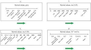
For many diseases (e.g., inflammation, demyelination, tumors, etc.) T1 and T2 are increased, but in other conditions, including, for example, hemorrhage and iron deposition, T1, T2 and T2* are often decreased. Diffusion is frequently decreased in acute disease of the brain (infarction, infection) and in many tumors, but increased in other tumors and chronic disease.
For particular applications, it is useful to focus on the relevant tissues and changes in them in disease. Figure 2 illustrates normal values of T1, T2 and D* in the prostate as well as changes in these TPs in tumors. Primary prostate tumors are unusual in that they show a decrease in T1 and T2 (as well as the more common decrease in D* in tumors) (4,5). The size of the changes is larger in the PZ than in the TZ and the fractional change is greater for T2 and D* than it is for T1.
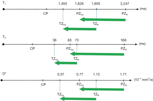
The signs and magnitudes of the changes in TPs as shown in Figure 2 are also important for scMRI. If concurrent changes in different TPs are present (which is usually the case), there is an opportunity to use appropriate sequences and image processing to make each of the changes in TP contribute synergistically to the overall contrast of images irrespective of the sign of those changes. The magnitude of the changes in TPs is also important in assessing their relative importance as sources of contrast.
Fluid properties are important in imaging the brain, for example, and often establish the upper or lower points of the image display dynamic range. Partial volume effects between very long T1 and T2 CSF and normal tissues may simulate increases in T1 and T2 in tissue and thus lesions. For this reason, it is often useful if CSF signals are selectively reduced when heavily T2-weighted sequences are used. This can be done with techniques such as CSF nulling (T2-FLAIR sequence) and late echo subtraction (les) (MASDIR sequences). Ideally these techniques should not reduce contrast between the tissues of primary clinical interest.
Pulse sequences as TP-filters and the CCT
The central contrast problem
The central contrast problem in clinical MRI is to relate differences/changes in TPs such as Δρm, ΔT1, and ΔT2 (or fractional changes in these TPs , and ) (Table 1, left column) to differences/changes in signal S i.e., contrast Cab = ΔS (or fractional contrast Cfr = ) as well as phase θ and differences in phase (Δθ) (Table 1, right column). This is done via knowledge of the relevant pulse sequences and pulse sequence parameters (Table 1, central column). Although the Bloch equations describing MRI relate S to TPs, the primary interest in clinical practice is in relating differences/changes in S (i.e., contrast) to differences/changes in TPs.
The conventional way of doing this is to use qualitative weighting. This designates a single TP as the one thought to be most responsible for the contrast of interest, and describes sequences and images accordingly as, for example, “T1-weighted”, “T2-weighted” and “diffusion-weighted”. However, contrast is often dependent on differences/changes in more than one of the ten TPs shown in Table 1. In addition, there are also at least six classes of pulse sequences and these display varying sensitivities to differences/changes in TPs. There are also differences within pulse sequence classes which depend on sequence parameters. This complexity leads to inconsistencies with qualitative weighting when only a single TP is used to describe the relationship between differences/changes in several TPs and the contrast they produce.
Problems with qualitative weighting
Examples of the problems encountered with the use of qualitative weighting include:
- A sequence which is T1-weighted in one application, for example showing contrast between white and gray matter in the brain, can be T2-weighted in other applications (such as showing contrast between normal and diseased tissue in the Achilles tendon) even though the sequence is still usually described as a T1-weighted image in this particular application (Figure 3).
- T2-FLAIR sequences are highly T2-weighted for the brain but are simultaneously highly T1-weighted for CSF.
- “Diffusion weighted” sequences may be more T2-weighted than diffusion weighted.
- Although reducing TE is said to reduce T2-weighting, subtracted ultrashort TE (UTE) sequences with UTEs (i.e., 8 ms) can be highly T2-weighted.
- “Fluid sensitive” sequences used in the musculoskeletal system are insensitive to fluids such as pore water and matrix bound water in cortical bone. On the other hand, UTE subtraction sequences that are sensitive to pore and matrix bound water are insensitive to joint and bursal fluid.
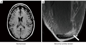
These and other inconsistencies complicate the use of qualitative weighting for image interpretation in clinical practice, and limit its usefulness for understanding more complex sequences as well as developing new applications of sequences for clinical MRI.
In order to resolve these problems, it is necessary to recognize the fact that several different TPs usually determine contrast with most pulse sequences, and provide specific relationships between difference/changes in TPs and difference/changes in signal (i.e., contrast) with these sequences. This is outlined in the next sections.
The spin echo (SE) sequence
The usual explanation of image signal and contrast with the SE sequence utilizes the Bloch equations. Firstly, it follows longitudinal magnetization (MZ) over time TR, and secondly follows transverse magnetization (MXY) after the application of a 90° pulse for further time TE (Figure 4). Contrast between two tissues such as P with a shorter T1 and T2, and Q with a longer T1 and T2, is shown by the difference in MXY at the time of data collection (dc) at TE as in Figure 4.
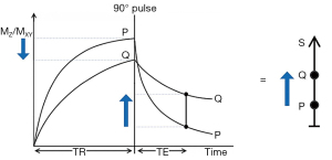
The voxel signal S for a SE sequence is derived from the simplified Bloch equations so that:
where K is a scaling function, ρm is the mobile proton density, and t is time. T1 and T2 are time constants. Eq. [1] describes ρm in the first segment, recovery of longitudinal magnetization (MZ) over time in the second segment (which is in parentheses), and decay of transverse magnetization (MXY) over time in the third segment. The equations in the second and third segments are of the forms y=1-e-x and y=e-x respectively.
Eq. [1] describes the signal of a tissue (with specific values of T1 and T2) for a SE pulse sequence for specific values of TR and TE. To compare different tissues, at least two curves need to be plotted as in Figure 4.
It is useful to replace the variable t in Eq. [1] by the constant times of the SE sequence TR and TE, and to treat the two time constants T1 and T2 in Eq. [1] as variables. This changes Eq. [1] to:
or:
where the signals for the three segments Sρm, ST1 and ST2 are given by:
The second and third segments in Eq. [2] are of the forms y=1-e-1/x and y=e-1/x respectively (since T1 and T2 are now variables). These forms are quite different from the forms y=1-e-x and y=e-x shown in the second and third segments of the Bloch equations in Eq. [1].
The three segments of Eqs. [2-4] have the features of a linear or exponential filter for ρm, [depending on whether the X axis is linear or natural logarithmic (ln)], a low pass filter for T1 and a high pass filter for T2 (Figure 5).
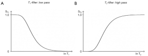
The signal levels on images are given by Eqs. [2-4] for ρm, ST1 and ST2, and correspond to the signal or brightness of tissues seen on images.
Eqs. [2-4] can be plotted using a linear or a logarithmic X axis. When using a linear axis, changes in X (i.e., changes in ρm, T1 or T2) represent absolute differences in TPs. When using a logarithmic X axis, small changes in X (i.e., Δln ρm, Δln T1 and Δln T2 represent fractional changes in TPs because for small differences between a and b, .
Absolute contrast (Cab) or difference in signal ΔST1 produced by a difference between the T1s of two tissues P and Q is shown in Figure 6 using a ln X axis. A positive change from P to Q of Δln T1 along the X axis produces a negative change from P to Q along the Y axis, or negative change in signal ΔST1 i.e., contrast Cab=ΔST1.
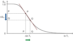
The equation for Cab for small changes in ΔT1 and ΔST1 using a linear X axis is:
where is the first partial derivative of the T1-filter with respect to T1, or the slope of the T1-filter, x=multiplied, and ΔT1 is the change in T1 using a linear X axis.
Using a ln X axis, and noting that for small changes in T1, and that , where x is a variable, Eq. [5] becomes:
where is the slope of the filter, or the first partial derivative with respect to lnT1 (when using a ln X axis), x=multiplied in this and subsequence equations, and is the fractional change in T1 as in Figure 6. For the T1 filter, positive change from P to Q along the X axis results in negative change from P to Q along the Y axis i.e., negative contrast Cab. The slope of the curve, which is the sequence weighting for the T1 segment, is negative.
For the T2 filter (Figure 7), positive change from P to Q along the X axis results in positive change ΔST2 = Cab from P to Q along the Y axis i.e., positive contrast. The slope of the filter, which is the sequence weighting for the T2 segment, is positive.
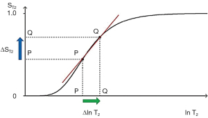
Solving for the situation when the second derivative of the TP-filter is equal to zero yields the TP value where the slope of the filter, and therefore the contrast, is highest. For the T1- and T2-filters, the slope is greatest at TR=T1 and TE=T2 when using a ln X axis, and at TR=2T1 and TE=2T2 when using a linear X axis.
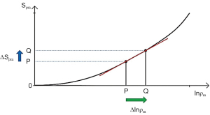
A similar pattern for contrast applies to ρm where an increase in ρm and positive slope of the ρm-filter produce positive contrast ΔSρm=Cab (Figure 8).
For fractional contrast Cfr=ΔS/S (rather than Cab=ΔS), Eqs. [5,6] are divided by ST1 and ST2 respectively for non-zero values of ST1 and ST2.
So, for T1 using a ln X axis:
and for T2 using a ln X axis:
The filters can be considered separately (i.e., a univariate model for each TP alone, as above), or be combined in a multivariate model. This shows the contributions of the sequence weightings and changes in each TPs to overall contrast for each of ρm, T1 and T2 in the SE sequence and is illustrated in Figure 9.

From Eqs. [3,4] for small change in Δρm, ΔT1 and ΔT2, and using a ln X axis, the product rule from differential calculus gives:
Normalizing Eq. [9] by dividing it by S and using Eq. [3], for non-zero values of S, Sρm, ST1 and ST2, Cfr is given by:
Thus the contributions of the TPs to the overall contrast Cfr are for each TP its sequence weighting multiplied by the fractional change in the TP. The relative contributions of each TP to sequence and image weighting can be calculated and expressed as ratios.
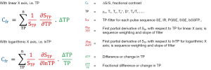
From Eq. [10] the overall fractional contrast Cfr using a ln X axis is given by:
where is the sequence weighting for the TP and is the fractional change in the TP. This is one form of the CCT for MRI and its corollaries which are shown in Figure 10. Using a ln X axis, the contrast for each TP is the normalized first partial derivative with respect to lnTP multiplied by the fractional change in TP. The total fractional contrast Cfr is the algebraic sum of the contributions to contrast from each TP. For T1 and T2, if both fractional contrasts are positive, or if both are negative, a synergistic contribution to overall Cfr results. If one TP contrast is negative and the other is positive a reduction in overall Cfr results. Thus, to achieve synergistic contrast, contributions to contrast of the same sign are sought from each of the relevant TPs to make their effects complementary.
The IR sequence
The IR sequence has an additional T1-filter (segment) to those of the SE sequence shown in Figure 9 for which:
This T1-filter is shown in phase-sensitive (ps) reconstructed form in Figure 11A and in magnitude (m) reconstructed form in Figure 11B.

When TI is increased, the T1-filter shifts to the right as show for the m form in Figure 12. Figure 12A shows the IR T1-filter with a short TIs (e.g., the STIR sequence) for the brain where gray matter (G) has a higher signal than white matter (W). The slope of the filter between W and G is strongly positive. When TI is increased to an intermediate TIi as in Figure 12B with W and G fixed in the same position on the ln X axis, W now has a higher signal than G. The slope of the filter between them is strongly negative. When TIi is increased further to a long TIi as in Figure 12C, W is slightly higher signal than G and the slope of the filter between them is negative but of smaller size than in Figure 12B. The sequence weighting, which is the slope or first partial derivative of the filter is highly positive in (A), highly negative in (B) and slightly negative in (C) using a short TIs (A), an intermediate TIi (B) and a long TIl (C) respectively. When TR>>T1 with the IR sequence the other T1 filter (1-e-TR/T1) becomes ~1 and the main determinant of contrast is the (1-2e-TI/T1) filter.

The pulsed gradient spin echo (PGSE) sequence
For diffusion using the PGSE sequence an additional segment is added to those shown in Figure 9 for the SE sequence and is illustrated in Figure 13 under D*. The extra segment is the D*-filter which has the form of an exponential decay with its signal SD* given by:
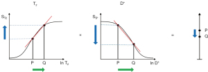
b is the diffusion sensitivity parameter and D* is the apparent diffusion coefficient. Significant D*-weighting requires a long TE with the PGSE sequence using present day clinical scanners. This is to provide time for the two pulsed diffusion gradients to be applied before and after the inversion pulse of the SE sequence. The long TE necessary for this creates T2-weighting and so the sequence simultaneously has positive T2-weighting (positive slope of the T2-filter shown in Figure 13 under T2), and negative D*-weighting (negative slope of the D*-filter shown in Figure 13 under D*). Positive change ΔT2 from P to Q along the X axis (horizontal green arrow) produces positive T2 contrast (positive vertical blue arrow). Positive change ΔD* from P to Q along the X axis produces negative D* contrast (negative vertical blue arrow). The result of the opposed T2 and D* contrasts produced in this way is overall low negative contrast (negative vertical blue arrow on the right). This is the case in many tissues where disease produces an increase in both T2 and D*, and the resulting opposed diffusion and T2 contrasts produce low overall contrast.
Figure 14 shows the situation when T2 is increased from P to Q under T2, and D* is decreased from P to Q under D* (rather than increased as in Figure 13). The changes in T2 and D* both result in positive contrast (blue arrows) and the algebraic sum of these is synergistic and produces high positive contrast (vertical blue arrow on right). In this situation, the PGSE T2 and diffusion weightings work together with the changes in T2 and D* to produce synergistic contrast.

The spoiled gradient echo (SGE) sequence
The SGE sequence has a T1-filter which is affected by two pulse sequence parameters TR and the flip angle α {Eq. [14]}. The filter appears the same as the SE sequence for flip angle α=90° but as α is reduced, the curve flattens and there is less T1 sequence weighting for a given value of TR (Figure 15).
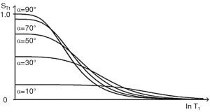
S is signal, α is the flip angle, and TR is repetition time. The flip angle to maximize signal αs is determined by setting the first derivative of Eq. [14] to zero. The flip angle to maximize contrast αc is determined by setting the second derivative of Eq. [14] to zero.
Values of αs, to maximize signal and to αc to maximize contrast are shown in Figure 16 for different values of TR and T1.
With the SGE sequence, the T2-filter of the SE sequence becomes a T2*-filter and includes additional effects from susceptibility which make T2* less than T2, and chemical shift. Chemical shift effects are modelled by including phase differences for water and fat and taking the vector sum and difference of these as with the Dixon technique.
Features of TP-filters
Features of the TP-filters approach include:
- Placement of TPs along the X axis, and the use of both ln and linear scales along this axis.
- Placement of signal S, or Q along the Y axis and use of both linear and logarithmic scales for this.
- Use of both absolute contrast Cab and fractional contrast Cfr.
- Designation of the slope or first derivative of the TP-filter (or normalized slope of the TP-filter) as sequence weighting and calculation of this slope both for linear and ln X axes.
- The use of second derivatives of the TP-filter and points of inflection to calculate values of sequence parameters (e.g., TR=T1, TE=T2 with ln X axes) to maximize Cab.
- Allocation of signs (positive or negative) to each of signal, contrast, image weighting, sequence weighting and TP differences/changes. This makes it possible to understand contrast and weighting in semi-quantitative and quantitative terms.
- Separation of sequence and image weighting with calculation of sequence and image weighting ratios to determine the relative contributions of different TPs to sequence weighting and image weighting.
- Ability to deal with the situation where a single TP (e.g., T1) is affected by two pulse sequence parameters (TR, a), or a single pulse sequence parameter (e.g., TE) has effects on two TPs (e.g., T2 and D*).
- TP values cover the full extent experienced in clinical practice so the graphics provide a complete representation of the contrast and weighting that is seen on images.
- The same approach can be used for sequence preparations as well as complete pulse sequences.
- Although developed here primarily for ρm, T1, T2, D* and T2*. The TP-filters approach is also applicable to other TPs.
Features of the CCT and its corollaries
First and foremost, unlike conventional qualitative weighting which only utilizes a single tissue TP to explain contrast, the CCT makes it possible to deal with two or more TPs and understand their separate and combined contributions to contrast. As a result, use of the CCT resolves many of the inconsistencies associated with the use of conventional qualitative weighting. Resolution of one of these inconsistencies is shown in Figure 17 which explains the fact that a SE sequence which is T1-weighted for the brain is T2-weighted for disease in the Achilles tendon, as was illustrated in Figure 3. It also makes it possible to understand how T2 and D* contrast behave individually and how they interact with each other in the PGSE sequence (Figures 13,14).

The CCT formalizes the relationship between differences/changes in TPs and fractional contrast, Cfr (Figure 10). It is in two parts. Firstly, for each TP the fractional contrast generated is the normalized product of sequence weighting (partial derivative of the TP-filter either with respect to the TP or lnTP) multiplied by the change in TP, or the fractional change in TP. The second part is the algebraic sum of the fractional contrasts generated by each TP which is the overall fractional contrast Cfr. For signal S, the CCT and its corollaries are derived from the Bloch equations for ρm, T1 and T2 and the Torrey equations which add diffusion D*. The CCT is used in graphical form in this paper.
The CCT can be used in qualitative form to determine which single TP of several is most responsible for contrast for given changes in the TPs and a specific pulse sequence. It is the TP with the largest Cfr. It can also be used in semi-quantitative or graphical form where the sign of differences/changes in TP and their relative magnitudes are considered. It can also be used in quantitative form where sequence and image weighting ratios express in percentages the relative contributions of each TP to sequence weighting and to image weighting using the equations:
The sequence weighting ratio sWr describes the relative weighting of the TPs within a sequence. The image weighting ratio (iWr) uses the sequence weighting ratio and combines it with differences/changes in each TP to describe their relative effects on the contrast of the image. This is an important difference. The sequence T1-filter may be steeper than its T2-filter meaning that it is more T1-weighted than it is T2-weighted for particular values of T1 and T2. However, if disease results in a larger change in T2 than in T1, contrast on the image can be dominated by the T2 change not the T1 change, so that the image has a dominant T2-weighting in spite of the fact that the sequence has a dominant T1-weighting.
The CCT and its corollaries employ the small change approximation of differential calculus. This is applicable, in particular, to the detection of effects due to small changes in TPs which is appropriate for demonstration of subtle disease. When large changes are present the small change approximation may lead to errors, but this is a known issue and is usually not a problem in clinical practice since large changes are usually easy to detect.
The use of fractional contrast involves normalization by the TP filter signals STP as well as the overall signal S. If one or more of these is zero, or close to zero when image noise is taken into account, values may take the form 1/0 and be uninterpretable. It means that fractional contrast is only valid between certain limits.
It is also not obvious which of absolute contrast Cab or fractional contrast Cfr best represent what is visually perceived by human observers and therefore provides the more appropriate model for understanding contrast. As a result, in this paper consideration is given to both forms of contrast.
The signal and contrast produced by sequences are subject to changes in window width and level performed by the observer. This has an effect on the perception of contrast and also needs consideration.
MASDIR pulse sequences
Development of the MASDIR sequence
The first combination of two IR sequences to form a single sequence was described in 1985 (6). This was the use of two successive inversion pulses to suppress signal from fluid then fat and was applied in the brain and body as the Double IR (DIR) sequence. Its use was extended to suppression of either white or gray matter signals as well as CSF in 1994 (7). More recently, in 2010 the Magnetization Prepared 2 Rapid Acquisition Gradient Echo (MP2RAGE) sequence was described (8). It multiplies two IR sequences together and normalizes them.
Groups of MASDIR sequences
A classification of MASDIR sequences is shown in Table 2. They are divided into: (i) multiplied, (ii) added, (iii) subtracted, and (iv) divided. Fitted IR (FIR) sequences are treated as a separate category. There are many types of MASDIR sequences and these are discussed briefly below. Subsequent sections describe some of them in more detail.
Table 2
| Groups of MASDIR sequences | Expansion of MASDIR sequence acronyms |
|---|---|
| MIR | Multiplied IR |
| DIR | Double IR (mTIl × mTIs/i) |
| MP2RAGE | Magnetization Prepared 2 Rapid Acquisition Gradient Echo (psTIl × psTIi) (also added and divided) |
| AIR | Added IR |
| AIR | Added IR (mTIs/i/l + mTIs/i/l) |
| A1IR | Added IR (psTIs/i/l + mTIs/i/l) |
| A1IRES | AIR Added IR Echo Subtraction |
| S1AIR | Subtracted, Added IR |
| SIR | Subtracted IR |
| SIR, rSIR | Subtracted IR (mTIs/i/l - mTIs/i/l), reverse SIR |
| SIRES, rSIRES | Subtracted IR Echo Subtraction, reverse SIRES |
| SIREDS, rSIREDS | Subtracted IR Echo Diffusion Subtraction, reverse SIREDS |
| SIRGES, rSIRGES | Subtraction IR Gradient Echo Subtraction, reverse SIRGES |
| SIRDGES, rSIRDGES | Subtraction IR Diffusion and Gradient Echo Subtraction, reverse SIRDGES |
| *DESIRE, STAIRES | Double Echo Sliding IR, Short TR Adiabatic pulse prepared IR (TR x mTIi/s) Echo Subtraction |
| *shMOLLI | Shortened Modified Look-Locker Inversion Recovery |
| S1IR | Subtracted IR (psTIs/i/l − mTIs/i/l) |
| S2IR | Subtracted SIR |
| IRES | IR Echo Subtraction |
| STIRES | Short TI IR Echo Subtraction |
| dIR | Divided IR |
| dSIR, drSIR | Divided SIR, divided reverse SIR |
| dSIRES, drSIRES | Divided SIRES, divided reverse SIRES |
| dSIREDS, drSIREDS | Divided SIREDS, divided reverse SIREDS |
| dSIRGES, drSIRGES | Divided SIRGES, divided reverse SIRGES |
| dSIRDGES, drSIRDGES | Divided SIRDGES, divided reverse SIRDGES |
| FLAWS div | Fluid and white matter suppressed, divided |
| FLAWS hc, FLAWS hco | FLAWS high contrast, FLAWS high contrast opposed |
| FIR | Fitted IR (multiple TIs) |
| MPnRAGE | Magnetization Prepared Rapid Acquisition Gradient Echo |
| *shMOLLI | Shortened Modified Look-Locker Inversion Recovery |
| *DESIRE | Double Echo Sliding IR |
*, included in both the subtracted and fitted categories. MASDIR, multiplied, added, subtracted and/or divided inversion recovery.
Multiplied IR (MIR) sequences
MIR sequences include DIR and MP2RAGE as mentioned above.
Added IR (AIR and A1IR) sequences
One group of AIR sequences adds two magnitude reconstructed sequences with different TIs and is used with subtraction and division (see below). Another group of sequences (A1IR) use a single TI with images reconstructed in ps and m forms. Addition of these two sequences shows shorter T1 tissues and suppresses the signal from longer T1 tissues and fluids. The A1IRES sequence supplements this by Echo Subtraction (ES, see later) and so adds a T2-filter reducing the signal from longer T2 tissues and fluids to provide a combined short T1 short T2-filter. The Subtracted AIR (S1AIR) sequence subtracts a longer TI image from a shorter one to selectively show a specific range of short T1 tissues.
SIR sequences
Eight subgroups of SIR sequences are included in Table 2. The first five use subtraction of a longer TI image from a shorter TI one (or vice versa as the reversed or r form). They start with the basic sequence (SIR), add T2-weighting to it as the SIRES sequence, and then add D*-weighting to this as the SIREDS sequence. The SE segment of the SIRES sequence is substituted by a gradient echo to produce the SIRGES sequence. This can have added to it diffusion weighting as the SIRDGES sequence.
The sixth group includes Double Echo Sliding Inversion REcovery (DESIRE) (9) which uses a sliding TI window to obtain many IR images with different TIs followed by a UTE data collection (dc) and ES, and the Short TR Adiabatic IR Echo Subtraction (STAIRES) (10) sequence. This sequence multiplies a very short TR segment by a short intermediate TIs segment to reduce to zero, or nearly zero, long T1 and T2 signals from tissues with a wide range of T1s. It is used with UTE dcs to provide selective imaging of ultrashort T2 tissues. This is followed by ES to reduce to zero the signal from any long T2 tissues which are not completely nulled. Both the DESIRE and STAIRES sequences can be used selectively to image myelin and other ultrashort T2 tissues.
The seventh group uses the same TI and subtracts a ps image from a m image once (S1IR), or twice (S2IR) with different TIs, for example, to selectively show a fluid or tissue.
The eighth group of SIR sequences is a basic IR Echo Subtraction (IRES), and the STIRES (STIR and ES) sequence which nulls shorter T1 white adipose tissue (WAT) and uses Dixon subtraction of out-of-phase images from in-phase images to selectively show lipid present in BAT as a result of its longer T1 compared to the T1 of lipid in WAT.
Divided IR (dIR) sequences
A central issue with division of IR sequences is the behaviour of the filter if or when the denominator takes a value of zero. This potentially leads to infinite values of the filter. Even if zero values are avoided, there are values when the denominator approaches zero and division becomes unreliable as a result of noise and artifacts.
The problem can largely be avoided with two SIR images by making the denominator the addition of the signals in the two images. The filters have different TIs, and using magnitude reconstruction, the sum of them in the denominator is non-zero. Division also normalizes the sequence so that the effects of ρm and T2 are reduced or eliminated, as are those due to receiver coil inhomogeneity.
Inclusion of division is the main advance over the previous formulation of MASTIR (Multiplied, Added, Subtracted and/or fiTted IR) sequences which are now described as MASDIR sequences. This includes each of the four basic operations of arithmetic and regards the fitted category (i.e., the Fitted IR, FIR sequences) as a separate mathematical operation.
Subtracted (SIR), Added (AIR) and Divided (dSIR) filters (univariate T1 models)
Two IR filters with different TIs are shown in Figure 18A. They are subtracted to give the SIR filter in Figure 18B. This T1-filter is steep in the X axis region between the inversion times, i.e., the middle Domain (mD). The two sequences in Figure 18A can also be added as the AIR sequence which is shown in Figure 18C where there are higher signal and higher slopes outside of the mD. The mD in Figure 18C has a low signal with a nearly linear slightly downward sloping curve.

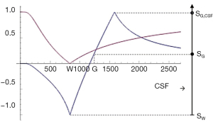
Figure 19A shows the T1-filter for the divided Subtracted IR (dSIR) filter in which the SIR filter in Figure 18B is divided by the AIR filter in Figure 18C. The dSIR filter shows a very highly sloping positive mD.

Figure 19B compares the contrast from the short TI T1-filter, STIs (pink) which is that of a conventional intermediate TIi IR sequence such as magnetization prepared rapid acquisition gradient echo (MP-RAGE) to that from the SIR filter (blue). The vertical pink and blue arrows on the right show that the contrast produced by the SIR filter is about double that produced by the STIs filter for the same change in T1 (horizontal green arrow across the mD).
Figure 19C compares the contrast produced by the short TI filter, STIs (pink) to that from the dSIR sequence (blue). For the same change in T1 (positive horizontal green arrow across the mD) the dSIR filter generates about five times the contrast produced by the STIs filter (vertical pink and blue arrows). As the second TI is moved closer to the first TI, the slope of the T1 tissue filter in the mD becomes steeper, and so the T1 dependent contrast in the mD increases. This is documented in Table 3. In this table, as ΔTI decreases from 90% to 13% the ratio of the contrast produced by the dSIR sequence to that produced by the conventional IR sequence increases from 5 to 20. The trade-off for this amplified contrast is a decreased mD where the sequence weighting and the contrast ratio is high. The mathematical basis for this is described in Appendix 1.
Table 3
| TIs (ms) | TIi (ms) | ΔTI | STIs contrast | SdSIR contrast | Ratio of SdSIR/STIs contrast | |
|---|---|---|---|---|---|---|
| ms | % | |||||
| 580 | 1,100 | 520 | 90 | 0.40 | 2.0 | 5 |
| 580 | 840 | 260 | 45 | 0.25 | 2.0 | 8 |
| 580 | 710 | 130 | 22 | 0.15 | 2.0 | 13 |
| 580 | 655 | 75 | 13 | 0.10 | 2.0 | 20 |
As TIi is reduced the mD narrows, ΔTI decreases and the signal for TIs at TIi (STIs value) decreases. The ratio of the dSIR contrast to the STIs contrast increases from 5 to 20, as ΔTI decreases from 90% to 13% when the mD narrows. dSIR, divided subtracted IR.
Figure 20A illustrates the rSIR filter and shows the same two filters for STIs and STIi as in Figure 18A. In Figure 20B the reverse (r) subtraction rSIR filter is shown. This has a negative slope in the mD. In Figure 20C addition of the two original filters gives the AIR filter as shown. Figure 21A shows the rSIR filter in Figure 20B divided by the AIR filter in Figure 20C to give the drSIR filter. This has a steeply sloping negative mD. Figure 21B shows a comparison of the STIi filter (pink) with the rSIR filter (blue) for a decrease in T1 (negative horizontal green arrow). The contrast produced by the rSIR filter is about twice that of the STIi filter (vertical pink and blue arrows on right). Figure 21C shows a comparison of the STIi filter (pink) with the drSIR filter (blue). The contrast produced by the drSIR filter is about five times greater than that from the STIi filter (pink and blue arrows on the right) as a result of using T1 synergistically to produce contrast 3–4 times.


The image processing for the sequences is shown in Table 4 for positive change in T1 (#1) and a negative change in T1 (#2). The two filters are processed in the same way. The SIR filter gives positive contrast in #1 and negative contrast in #2. The rSIR filter gives negative contrast in #1 and positive contrast in #2.
Table 4
| # | Sign of ΔT1 | Image processing | Examples |
|---|---|---|---|
| 1 | + | Row I (TIs): (Row I minus Row II) to give SIR, then r; (Row II minus Row I) to give rSIR, then ± d | Many diseases |
| Row II (TIi) | |||
| 2 | − | Row I (TIs): (Row I minus Row II) to give SIR, then r; (Row II minus Row I) to give rSIR, then ± d | Some hemorrhage, iron deposition, GBCA/MIOP accumulation |
| Row II (TIi) |
Changes in ΔTP (ΔT1) in disease can be negative (−) or positive (+). In most diseases, T1 is increased (+), but in hemorrhage, iron deposition and other diseases T1 is decreased (−). Image processing in #1 i.e., the subtraction (Row I minus Row II) produces positive T1 synergistic contrast with SIR processing, and negative T1 synergistic contrast with reversed rSIR processing. Image processing in #2 produces positive and negative T1 synergistic contrast with rSIR and SIR processing respectively. SIR, subtraction inversion revovery; rSIR, reverse SIR; d, division; GBCA, gadolinium based contrast agents; MIOP, magnetic iron oxide particles.
The mathematical basis for key features of the dSIR and drSIR filters including their near linearity, slope approximately equal to +/− ln 4/ΔTI and high sensitivity to small changes in T1 is included in the Appendix 1.
Including T2 and D*: Subtracted, Added and Divided IR sequences (multivariate models)
Division has also been incorporated as an option using AIR filters in the denominator to give dSIRES, dSIREDS, dSIRGES and dSIRDGES filters as well as their reversed (r) forms.
In order to create sequences with synergistic contrast, it is sometimes necessary to reverse the weighting of a conventional filter. ES is used to reverse the T2-weighting of the T2-filter. This is accomplished by the subtraction: short TE filter minus long TE filter as in Figure 22. Increases in T2 in the chosen domain for the T2-filter result in increased signal. For the ES filter, increase in T2 results in decreased signal. Thus, the T2-filter weighting has changed from positive to negative.

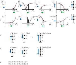
Row I of Figure 23 describes a filter with a short TI and a long TE resulting in positive contrast from the T1 and T2-filters [middle and right columns (B) and (C)]. Row II of Figure 23 shows an intermediate TI filter with negative contrast from both the T1 and T2-filters. Row II includes the subtraction: intermediate TIi short TE sequence minus intermediate TIi long TE sequence. Thus, ES reverses the sign of the conventional T2 filter. In Row III, the SIRES filter is created by the subtraction: Row I minus Row II which produces overall synergistic positive T1 and T2 contrast. Row IV shows the reversed subtraction rSIRES. Row V shows the divided dSIRES and drSIRES filters which result in further increase in T1 contrast as discussed previously.
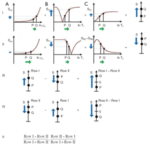
Diffusion subtraction (DS) is used to reverse the weighting of the D* tissue filter. This is accomplished by the subtraction: D*-filter with b=“0” minus D*-filter with a high b value as in Figure 24. For the short TE and b=“0” filter in Figure 24A, increase in D* results in no change. For the diffusion filter in Figure 24B, increase in D* results in negative contrast. For the subtracted D*-filter, increase in D* produces positive contrast.

The SIREDS filter (Figure 25) adds D* to the SIRES filter and includes DS to create synergistic T1, T2 and D* contrast. Row I in Figure 25 is a filter with a short TIs, long TE, and high b value resulting in positive synergistic contrast for increases in T1 and T2, and a decrease in D* as seen in some acute disease and many tumors. Row II in Figure 25 is a filter with negative synergistic contrast for increase in T1 and T2 and decrease in D*. Row II includes the subtraction: intermediate TIi, short TE, b=“0” filter minus intermediate TIi, short TE, high b value [i.e., ES and diffusion subtraction (EDS)]. Row III shows the subtraction: Row I minus Row II to give the SIREDS filter. Row IV shows the rSIREDS filter. The dSIREDS and drSIREDS filters are shown in Row V and increase T1-weighting as above.
The Fluid and White Matter Suppressed (FLAWS)sequence was originally described with TIs chosen to null the signal from fluid and from white matter and these were combined by multiplication and normalized as the uni form of FLAWS (11). It was related to the MP2RAGE sequence which also multiplies and normalizes two IR sequences using the sum of the squares of the sequence signals in the denominator. The FLAWS sequence has been extended to include subtraction and division with the sum of the two sequences IR in the form of FLAWShc (FLAWS high contrast) and FLAWShco (FLAWS high contrast opposed) sequences which employ subtraction (12). It thus has common features with the dSIR and drSIR sequences. The FLAWdiv sequence is the shorter TI IR image divided by the longer TI IR image. This may become problematic when the signal from the longer TI IR image is nulled. Both FLAWShc and FLAWShco typically use wide mDs (ΔTI=156% at 1.5T [11] and ΔTI=130% at 7T [12]), not narrow mDs as with dSIR and drSIR sequences (e.g., ΔTIs=19–43% in this paper), and show lower contrast as a consequence. The FLAWShc sequence does not show high signal white-gray matter boundaries as the dSIR sequence does as a consequence of its wide mD. Unlike the FLAWShc and FLAWShco sequences, the dSIR and drSIR sequences are also combined synergistically with T2 and D* sequence weightings.
FIR sequences
These obtain multiple IR images primarily for quantification of T1 [e.g., MPnRAGE (13) and shMOLLI (Shortened MOdified Look-Locker Imaging) (14)]. The DESIRE sequence can be used in this way but can also be used for selecting the best TI to null long T2 components in tissue or tissues with different T1s. The DESIRE sequence is included in both the subtraction and fitted categories.
scMRI
Synergistic contrast can arise in two main ways:
- A single TP can be used twice or more in a sequence. For example, T1 can be used in the T1 dependent TR segment of an IR sequence as well as the T1 dependent TI segment. T1 is also used twice in DIR sequences when two TI segments are multiplied together, and in the Subtracted IR (SIR) sequence when using the subtraction: short TIs segment minus intermediate TIi segment. The synergistic T1 contrast from the SIR sequence can be increased further by using T1 3–4 times in the form of dSIR and drSIR sequences.
Synergistic contrast may arise from repeated use of T2 when imaging ultrashort T2 tissues with an IR sequence using a long adiabatic inversion pulse to invert and null long T2 signals while ultrashort T2 tissues that are saturated by the inversion pulse recover, and following this after the 90° excitation pulse by ES. The two effects, firstly from the inversion pulse and nulling, and secondly from the decay in transverse magnetization produce synergistic negative contrast when there is an increase in T2 in ultrashort T2 tissues. - Two or more different TPs can also be used to produce synergistic contrast. Clinical pulse sequences have a basic structure consisting of ρm, T1, and T2 filters as seen in SE sequences. There are additional options which can be added such as those for T1 dependent inversion pulses and D* sensitization. In many circumstances ρm is a minor determinant of contrast and T1, T2, and D* are major determinants. The most common change in TPs in disease is concurrent increases in ρm, T1, T2. In this situation with the SE sequence, the contrast developed by an increase in T1 is negative while that developed by an increase in T2 is positive, so that simultaneous increases in T1 and T2 produce opposed contrast and the net, or overall, contrast is reduced. To avoid this problem, T1-weighted sequences use a short TE to minimize the opposed T2 contrast, and T2-weighted sequences use a long TR to minimize the opposed T1 contrast. The dominant source of contrast in the resulting sequences is then a single TP, i.e., T1 or T2 and the sequences are described as T1-weighted or T2-weighted respectively. They are not synergistic for T1 and T2 contrast.
In particular circumstances, such as certain forms of the STIR and the DIR sequences, the T1 contrast produced by an increase in T1 is positive, and so is the T2 contrast produced by an increase in T2. The effects of the concurrent increases in T1 and T2 are therefore synergistic and typically result in high positive lesion contrast.
The contrast produced above from (i) a single TP, or (ii) two or more different TPs can be supplemented by increasing or decreasing signals from certain normal tissues and/or fluids. There may be little contrast between high signal lesions and high signal fat, long T2 tissues, or fluids. Reduction in the normal signal from these latter tissues or fluids [using the same or different TPs as those used to create the original synergistic contrast in (i) and/or (ii)] can increase the contrast between the high signal lesions and the zero or low signal suppressed tissues and/or fluids. It may also result in a more appropriate dynamic range for the image.
In a tissue with a mixture of ultrashort T2 and long T2 tissues, for example, low abundance ultrashort T2 tissues may only become apparent if the more abundant signals from the long T2 tissues are reduced or suppressed. This also applies to edema in yellow bone marrow, where suppression of the more abundant fat signal may be necessary to show the lower concentration edema. Signals can also be increased for the same purpose.
The synergistic contrast produced in (i) and (ii) can also be supplemented by opposed contrast outside the region of interest.
One or both of mechanisms (i) and (ii) described above may be used in any one synergistic contrast sequence with, or without, supplementary synergistic contrast from suppression or increase of signals from normal tissues as well as the use of opposed contrast. Achievement of synergistic contrast requires a knowledge of the sign of sequence weighting of the TP-filters involved, as well as the sign of the change in each TP.
Image processing to achieve synergistic contrast
There are three situations within sequences where the ability to reverse the sign of the weighting of a filter of the sequence is important for achieving synergistic contrast. These are firstly, reversal of the sign of the T1 contrast produced by a change in T1 with IR sequences by using different TIs (together with m reconstruction). Secondly, reversal of the sign of T2 contrast produced by a change in T2 with SE T2-filter by the subtraction: shorter TE filter minus longer TE filter i.e., ES. Thirdly, reversal of the sign of diffusion contrast produced by the PGSE D*-filter using the subtraction: low b value (e.g., 0–20 s/mm2) filter minus high b value (e.g., 500–1,500 s/mm2) filter i.e., DS. This ability to change the sign of the sequence TP-filter and the resulting contrast for T1, T2 and D* is crucial for creating synergistic contrast from either positive or negative changes in each of T1, T2 and D* in disease.
In addition to changing the sign of the sequence weighting of a filter within a sequence as above, it is also possible to reverse the order of subtraction of two sequences, and so reverse the contrast produced by the sequences. This is reverse (r) subtraction.
Using the same change in a TP twice or more in the same sequence may result in higher synergistic contrast than just using it once. Using changes in different TPs may also be effective in increasing overall contrast. This is because T1, T2 and D* often change concurrently in disease and using synergistic contrast to exploit the lesion contrast developed by each of these TPs may result in higher overall contrast. These are approaches targeted at increasing sequence sensitivity.
Image processing also includes late (very long TE) echo acquisition of signal from long T2 fluids such as CSF. This can be helpful when CSF is at the top or bottom of the display dynamic range when white or gray matter would be preferred in this location. It is also of value in avoiding problems with partial volume effects simulating lesions.
It is also possible to specifically include image acquisitions for their use in image processing. This includes, for example, short TE sequences for subtraction from them of longer TE sequences.
Synergistic contrast can also be used to improve sequence specificity, for example, by using the reductions in both T1 and T2* produced by organic iron to provide high contrast visualization of its effects.
The main modification since the previous paper has been to include division in the image processing since it substantially increases T1 synergistic contrast, usually as a final option after subtraction of filters and reversed subtraction of sequences (Tables 5,6).
Table 5
| # | ΔTP | Image processing | Disease examples | |
|---|---|---|---|---|
| T1 | T2 | |||
| 1 | + | + | Row I (TIs) nil (with les); (I minus II) then r ± d | Common diseases |
| Row II (TIi) ES | ||||
| 2 | + | − | Row I (TIs) ES; (I minus II) then r ± d | |
| Row II (TIi) nil (with les) | ||||
| 3 | − | + | Row I (TIs) ES; (I minus II) then r ± d | |
| Row II (TIi) nil (with les) | ||||
| 4 | − | − | Row I (TIs) nil (with les); (I minus II) then r ± d | |
| Row II (TIi) ES | Some hemorrhage, iron deposition, GBCA/MIOP accumulation | |||
Changes in signs of ΔTP (ΔT1 and ΔT2) in disease, image processing to produce positive or negative T1 and T2 synergistic contrast, and disease examples. In #1 both T1 and T2 are increased, and Row I requires no processing except les. Row II uses ES. The subtraction (Row I minus Row II) produces a SIRES image. The reverse subtraction (r) produces a rSIRES image. Both can be divided to produce dSIRES and rSIRES images. The same principles apply to #2, 3 and 4. SIRES, subtracted IR echo subtraction; rSIRES, reverse SIRES; r, reverse; d, division; les, long echo subtraction; ES, echo subtraction; GBCA, gadolinium based contrast agent; MIOP, magnetic iron oxide particles; dSIRES, divided SIRES.
Table 6
| # | ΔTP | Image processing | Disease examples | ||
|---|---|---|---|---|---|
| ΔT1 | ΔT2 | ΔD* | |||
| 1 | + | + | + | Row I (TIs) DS (with les); (I minus II) then r ± d | Chronic disease, some tumors |
| Row II (TIi) ES (no D*) | |||||
| 2 | + | + | ‒ | Row I (TIs) nil (with les); (I minus II) then r ± d | Acute disease (infarction, infection), many tumors |
| Row II (TIi) EDS | |||||
| 3 | + | ‒ | + | Row I (TIs) EDS; (I minus II) then r ± d | |
| Row II (TIi) nil (with les) | |||||
| 4 | + | ‒ | ‒ | Row I (TIs) ES (no D*); (I minus II) then r ± d | |
| Row II (TIi) DS (with les) | |||||
| 5 | ‒ | + | + | Row I (TIs) ES (no D*); (I minus II) then r ± d | |
| Row II (TIi) DS (with les) | |||||
| 6 | ‒ | + | ‒ | Row I (TIs) EDS; (I minus II) then r ± d | |
| Row II (TIi) nil (with les) | |||||
| 7 | ‒ | ‒ | + | Row I (TIs) EDS; (I minus II) then r ± d | |
| Row II (TIi) nil (with les) | |||||
| 8 | ‒ | ‒ | ‒ | Row I (TIs) DS (with les) (I minus II) then r ± d | |
| Row II (TIi) ES (no D*) | |||||
Changes in ΔTP (ΔT1, ΔT2 and ΔD*) in disease, image processing to produce positive or negative T1, T2 and D* synergistic contrast, and disease examples. In #1 Row I DS is used with les. In Row II ES is used. The subtraction Row I minus Row II is performed followed by the reverse subtraction ±division. The same type of pattern applies to #2–8. SIREDS, subtracted IR echo diffusion subtraction; rSIREDS, reverse SIREDS; r, reverse; d, division; les, long echo subtraction; ES, echo subtraction; DS, diffusion subtraction; EDS, combined echo and diffusion subtraction.
Contrast at tissue boundaries
In the previous sections of this paper, contrast between two voxels has been considered, but there has been no reference to the space between voxels, or contrast at boundaries between two voxels.
In general terms, contrast detectability at boundaries between two voxels can be related to Cab=ΔS or Cfr=ΔS/S divided by the distance Δx between the voxels. Boundaries are more detectable when contrast is high and Δx is low, rather than in the opposite situation where contrast is low and Δx is high.
At a boundary between two pure tissues P and Q it is useful to define the tissue fraction f which is the proportion of the second tissue Q in a voxel containing a mixture of both tissues. The proportion of the other tissue P is then (1-f).
The T1 of the mixture of the two tissues (P and Q) can be expressed as a function.
where T1P,Q is the T1 of the mixture, T1P is the T1 of P, and T1Q is the T1 of Q. An example of this is shown in Figure 26 (upper row, column B).
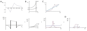
It is also useful to consider the change in tissue fraction with distance x. This is shown in Figure 26 (upper row, column C) and may be gradual corresponding to a low value of or more abrupt in parts corresponding to higher values of .
Using the chain rule from differential calculus, for T1
where is the change in fractional contrast with distance x, ST1 is the T1-filter signal, is a measure of detectable contrast, is the first partial derivative of ST1 with respect to T1 i.e., the sequence T1-weighting, is the change in T1 with tissue fraction f, and is the change in f with distance x. This is illustrated in Figure 26 (lower row).
If the sequence weighting is high as within the mD of a dSIR sequence is high (Table 7). In the brain is increased from white-gray matter to gray matter-CSF to white matter-CSF at boundaries between tissue fluids. increases as the transition from one tissue changes from gradual to abrupt.
Table 7
| Increasing T1 sequence weighting from upper to lower (below) | Increasing value from upper to lower | Increasing value from upper to lower |
| SGE | White-gray matter | Gradual |
| IR | Gray matter-CSF | Abrupt |
| SIR | White matter-CSF | |
| dSIR |
SGE, spoiled gradient echo; IR, inversion recovery; SIR, subtracted IR; dSIR, divided SIR; CSF, cerebrospinal fluid.
If one or more of the partial derivatives in Eq. [18] is zero, the tissue appears flat on the image. This can occur with “dark bone” imaging where the SGE sequence has a low flip angle and short TE, and is insensitive to T1 changes so that (but not to low ρm which accounts for the bone contrast). If the T1s of P and Q are the same , then no contrast results. If , i.e., there is no change in the proportions of the two tissues, no contrast results.
At a boundary between two tissues the actual T1 of the voxels with mixtures of tissues within them spans the range of T1 values between the two tissues. This is shown in Figure 27. If the T1-filter is such that a T1 value between those of the two tissues results in a high value of S, a high signal line results at the boundary between the two tissues, as seen in Figure 28. The width and location of the line is dependent on the slope of the filter and the gradient of T1 with f as well as the gradient of f with x as shown in Figure 26 (lower row). The high signal boundary at the white-gray matter boundary inside the brain in Figure 28 was obtained using a narrow mD.
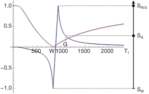
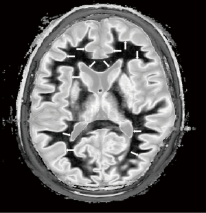
Figure 29 shows use of a wide mD filter in which maximum signal is reached with a T1 between those of gray matter and CSF. This arises from partial volume effects between gray matter and CSF, and produces a high signal boundary between gray matter and CSF outside of the brain as shown in Figure 30.
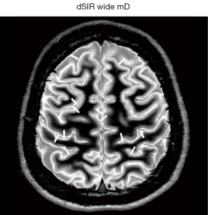
Boundaries can also be seen around lesions that increase their T1s beyond the T1 of the upper limit of the mD. The lesion then shows a high signal margin and a lower signal center because the T1 of the lesion is higher than the T1 resulting in maximum signal at the boundary.
The width and location of the boundary e.g., white-gray matter or gray matter-CSF can be changed by choice of mD and the width of the boundary can be changed, altering the slope and location of the maximum signal of the T1-filter. In general, wider mDs result in greater width of tissue boundaries.
The conventional wisdom on partial volume effects between tissues in the brain with SE dcs is that the signal of voxels containing two tissues such as white and gray matter is intermediate between those of the two constituent tissues. The appearances in Figures 28,30 are therefore counter-intuitive and difficult to explain without reference to TP-filters and the CCT.
High signal boundaries provide a useful basis for locating lesions as well as for segmentation of tissues and following changes in space in serial imaging studies as described in the next section.
Small change regimes
In general terms, there is often no particular premium in clinical MRI in demonstrating large changes with even greater contrast, so the emphasis with MASDIR sequences is on demonstrating lesions where there are only small changes in TPs with sufficient contrast for the images to be of diagnostic value. The emphasis has therefore been on imaging regimes to detect small changes and ideally monitor them over time to follow their natural history, and/or the effects of treatment.
Increased sensitization in the mD is accompanied by a decreased width of the mD. This combination is particularly appropriate for detecting small changes in T1 in specific tissues where high contrast can be produced by a small change in T1. Small changes from normal are commonly seen in earlier and more subtle forms of disease.
On MR images changes may be in signal or contrast, and in space, e.g., increase or decrease in size of normal structures, or in both signal/contrast and space.
Differences/changes in signal may be anatomical on single images, but may also include changes in space with growth and atrophy for example.
Perturbations in signal due to change in T1 occur with pre and post gadolinium-based contrast agent (GBCA) administration, inhalation of 100% O2, perfusion and angiography, as well as with fMRI.
Disease usually involves both changes in signal and space, but in some cases the changes in space are small and the situation can be treated as a change in signal.
The changes in signal and space from normal in a single image may change over time in serial studies as part of the natural history of the disease and/or the result of therapy. In the situation where changes are small, rigid body registration is well suited to accurately aligning images obtained on two or more occasions so that genuine changes can be distinguished from artefactual differences due to variation in slice alignment.
This has been performed with isotropic 3D SGE sequences and a system of interpretating images including distinguishing pure signal changes from spatial changes where possible has been described (15). 3D isotropic MASDIR sequences using MP-RAGE/BRAVO (BRAain VOlume) type data acquisitions with SIR/rSIR and or dSIR/drSIR image processing offer increased sensitivity to changes in contrast. They also offer high contrast, high resolution definition of boundaries to improve detection of changes in space. It is likely that this will be a significant application of MASDIR sequences.
Examples
Application of these principles can be seen in a case of multiple sclerosis (MS) (Figure 31). In the upper row the T2-FLAIR images demonstrate focal lesions in the pons and deep white matter of the left hemisphere. Normal white matter on the image is seen in the cerebellum and appears dark. The dSIR image shows very extensive change in white matter in the pons and adjacent cerebellum as high signal areas (arrows). These abnormalities are not seen on the T2-FLAIR image. Figure 32 is an enlarged version of the dSIR image in the upper row and Figure 33 is an enlarged version of the dSIR image in the lower row.
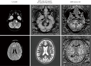
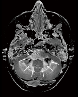
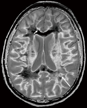
In the lower row of Figure 31 the T2-FLAIR image shows two focal lesions (arrows). These are seen on the dSIR image (Figure 31, lower row, right) and on the expanded image in Figure 33. There is extensive involvement of white matter which appears as higher signal regions compared with the normal white matter regions which are dark. High signal lines are seen at the boundaries between white matter and gray matter as well as between white matter and CSF. The lesion in the posterior deep white matter on the left (long white arrow) shows the “iceberg sign”. The abnormal area is surrounded by a high signal line (longer white arrow). Beyond the lesion, there are extensive areas of abnormal white matter which have signals greater than the normal level of black. These abnormal areas are not seen with the T2-FLAIR sequence.
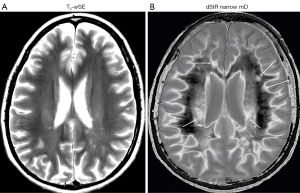
In the same case T2-wSE images are compared with dSIR images (Figure 34). No definite abnormality is seen on the T2-wSE image (Figure 34A) but three focal lesions are seen on the dSIR images (long arrows). The corticospinal tracts are also abnormal (short arrows) and there are areas of increased signal in the white matter (normal white matter appears black).
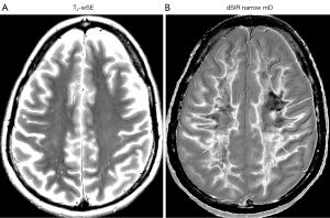
At a higher level (Figure 35), an obvious focal lesion is only seen with dSIR (long arrow). Abnormalities are seen in the corticospinal tracts (short arrows) and elsewhere in the white matter.
Practical issues
- A common cause of failure to show contrast with the SIR group of sequences is using an initial TI (e.g., to null white matter) which is too long. The nulling TI needs to be precisely targeting often at the transition between normal and abnormal T1 values.
- Another cause of failure to show high contrast with SIR type sequences is a ΔTI which is too wide. This provides broad coverage, but not high amplification for small changes in T1. ΔTI needs to be matched to the expected changes in T1.
- Low contrast may arise in a lesion if the T1 of the lesion is markedly increased, so that it “overshoots” the longer TI. It may then show mid-range signal (usually with a high signal boundary around it).
- High contrast may not be seen if the chosen mD does not allow for a significant increase/decrease in T1.
- There are a wide range of factors which affect the nulling TI. Fifteen of these are listed in Table 8 and one or more of them may account for a failure to null signal when expected.
Table 8
Causes of changes in the TI for nulling tissuesImaging techniques Changes in T1 Field strength B0 Change in T1 with age Different TRs Change in T1 with site in organ Different recovery times (with different TIs) Change in T1 with disease Efficiency of B1 pulse Change in T1 with contrast agents Inhomogeneity of B1 Change in T1 with 100% O2 inhalation Data collection e.g., gradient echo vs. SE Change in T1 with temperature Fast recovery Change in T1 with formalin fixation Fat saturation Uninverted ultrashort T2 species Decrease in observed/effective T1 due to magnetization transfer SE, spin echo. - Another problem may be that contrast is already high, and trying to show a further increase with SIR type sequences or the addition of T2 with SIRES type sequences may be difficult.
- There are advantages in specifically matching the initial nulling T1 and change in T1 with disease to ΔTI for sign and size of change as far as possible to take advantage of the near linear relationship between dSIR and drSIR signals and T1 as described in the Appendix 1.
- Not using les with SIRES and rSIRES means that CSF signal may be at the top or bottom of the display gray scale range. This may produce partial volume effects and make lesions less obvious.
- For SIR sequences the prostate is in many ways a mirror reflection of the brain. In disease, T1 and T2 are reduced. It is therefore useful to start with the longest T1 tissue PZ and use rSIR filters and work towards the shorter T1 TZ, and beyond this the shorter T1 of capsular tissue to establish nulling values of TI for the PZ and TZ.
- The location of boundaries with SIR and dSIR sequences i.e., whether they are internal or external to the cortex of the brain provides a reliable indication of whether the second TI is too short or too long.
- Partial volume effects at high signal boundaries may simulate lesions.
- Misregistration of images may produce high and low signal boundaries.
Discussion
The paper summarizes advances in TP-filters and the CCT, MASDIR sequences, and scMRI and uses concepts from each of these to develop a formalism for understanding contrast at tissue boundaries, small change regimes and a method for T1 quantitation. In images of MS, the archetypal disease for neuroinflammation, this combination outclasses the gold standard sequences T2-FLAIR and T2-wSE. The approaches are likely to have significant applications in brain, body and musculoskeletal systems.
The work has a mathematical basis using differential calculus to understand TP-filters and the CCT, as well as contrast at boundaries. The basic operations of arithmetic, namely multiplication, addition, subtraction and division are used to combine IR sequences. The graphics used to understand contrast is accessible using a basic level mathematical App such as WolframAlpha.
In the development of MRI many aspects such as image acquisition, reconstruction, processing and quantitation have primarily been the domain of physicists and other scientists. However, image contrast and clinical application of it has usually been the domain of radiologists and other clinicians. This latter activity involving sequence preparations, basic acquisitions and image processing has been an area where radiologists and clinicians can make a specific contribution to clinical MRI.
The illustrated examples highlight the brain since historically this is where clinical MRI began with concepts developed for the brain subsequently applied to the body, musculoskeletal system and cardiovascular system as well as to children. Normal white and gray matter provide an obvious point of reference for assessing contrast between two tissues, and the concepts for differentiating them can be applied to differentiating two other tissues i.e., normal and abnormal.
Prostate tumors in the peripheral and transitional zones are an interesting example where the T1 and T2 of tumors is decreased rather than increased (which is the common pattern elsewhere in the nervous system and body). This approach is in many ways a mirror reflection of what has been done in the brain. The baseline tissue is the long T1 PZ followed by the shorter T1 PZ (Figure 2). Reductions in T1 are seen in tumors so rSIR and rdSIR are used primarily rather than SIR and dSIR as in the brain.
There are a number of aspects to this work which appear counter-intuitive:
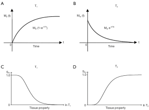
- In the Bloch equations for the SE sequence, the TP-filters approach assigns the variable time two constant values TR and TE, and treats the two time constants T1 and T2 as variables. The resulting filters which describe T1 and T2 effects on MRI images have the opposite slopes to those shown for T1 and T2 in graphical representations of the Bloch equations (Figure 36). Thus, instead of T1 describing an increasing exponential, the T1-filter describes a decreasing function (A and C, in the T1 column). Instead of T2 describing a decreasing exponential decay, the T2-filter takes the form of an increasing sigmoid function (B and D, in the T2 column). This can be a source of confusion.
- The application of commonly used MASDIR sequences also appears counter-intuitive. In the brain, to visualize white matter, the first step with the SIR sequence is to use a TI to null it. The next step is to null other tissues (e.g., abnormal tissues) with T1s close to that of white matter. Following this, the remaining signal is subtracted one way, and then the other way. What signal is left can be divided and further subtractions and reversals may follow for T2 and D*. After these operations, it seems unlikely that any useful signal will be left, or at best it will have a low SNR and not be of diagnostic use. The impetus to acquire nulled IR sequences and image process them in the way described came from mathematical modelling, not empirical observations of images.
- The sequence can also be counter-intuitive as far as tissue boundaries are concerned. The accepted view for partial volume effects at boundaries between white and gray matter, as well as between gray matter and CSF, is that their signal intensity is intermediate between those of the tissues or fluids involved. However, SIR and dSIR images often show boundaries between tissues with signals much higher than those of either of the constituent tissues or fluids.
- It also seems improbable that it is possible to achieve 5–15 times the contrast of already high contrast conventional intermediate TI IR sequences such as MP-RAGE and IR FSE.
- It is also possible to obtain T1 values directly from acquired dSIR and drSIR images without having to create T1 maps. The maps have the same high contrast and high spatial resolution as the original images.
- The signal intensities of CSF are often intermediate rather than high as in T2-wSE sequences, or low as in T1-weighted SGE or SE and T2-FLAIR sequences and this can undermine belief in the integrity of the imaging process.
- Very highly T1-weighted SIR and dSIR sequences look “T2-weighted” in that gray matter has a higher signal than white matter as is the case with T2-wSE sequences.
Resolution of these issues often follows from use of TP-filter graphics rather than the use of conventional qualitative weighting. As a result, understanding of contrast produced by MASDIR sequences can be easier for newcomers to the field than for experienced practitioners who may have to become accustomed to quite new appearances of images and unlearn traditional explanations for MR appearances that have taken them years to acquire.
Acknowledgments
The authors thank Dr. Nivedita Agarwal for providing Figure S1.
Funding: This work was supported by National Institutes of Health (Nos. R01AR062581, R01AR068987, R01AR079484 and R21AR075851), the VA Clinical Science Research & Development Service (No. I01CX002211), and GE Healthcare (Nos A-31, A-32 and A-33) as well as from Kānoa-RDU, New Zealand and Trust Tairāwhiti, New Zealand.
Footnote
Conflicts of Interest: All authors have completed the ICMJE uniform disclosure form (available at https://qims.amegroups.com/article/view/10.21037/qims-22-394/coif). JD serves as an unpaid editorial board member of Quantitative Imaging in Medicine and Surgery. GMB is a consultant to Magnetica. The other authors have no conflicts of interest to declare.
Ethical Statement: The authors are accountable for all aspects of the work in ensuring that questions related to the accuracy or integrity of any part of the work are appropriately investigated and resolved.
Open Access Statement: This is an Open Access article distributed in accordance with the Creative Commons Attribution-NonCommercial-NoDerivs 4.0 International License (CC BY-NC-ND 4.0), which permits the non-commercial replication and distribution of the article with the strict proviso that no changes or edits are made and the original work is properly cited (including links to both the formal publication through the relevant DOI and the license). See: https://creativecommons.org/licenses/by-nc-nd/4.0/.
References
- Young IR, Szeverenyi NM, Du J, Bydder GM. Pulse sequences as tissue property filters (TP-filters): a way of understanding the signal, contrast and weighting of magnetic resonance images. Quant Imaging Med Surg 2020;10:1080-120. [Crossref] [PubMed]
- Ma YJ, Fan S, Shao H, Du J, Szeverenyi NM, Young IR, Bydder GM. Use of Multiplied, Added, Subtracted and/or FiTted Inversion Recovery (MASTIR) pulse sequences. Quant Imaging Med Surg 2020;10:1334-69. [Crossref] [PubMed]
- Ma YJ, Shao H, Fan S, Lu X, Du J, Young IR, Bydder GM. New options for increasing the sensitivity, specificity and scope of synergistic contrast magnetic resonance imaging (scMRI) using Multiplied, Added, Subtracted and/or FiTted (MASTIR) pulse sequences. Quant Imaging Med Surg 2020;10:2030-65. [Crossref] [PubMed]
- Yu AC, Badve C, Ponsky LE, Pahwa S, Dastmalchian S, Rogers M, Jiang Y, Margevicius S, Schluchter M, Tabayoyong W, Abouassaly R, McGivney D, Griswold MA, Gulani V. Development of a Combined MR Fingerprinting and Diffusion Examination for Prostate Cancer. Radiology 2017;283:729-38. [Crossref] [PubMed]
- Panda A, Obmann VC, Lo WC, Margevicius S, Jiang Y, Schluchter M, Patel IJ, Nakamoto D, Badve C, Griswold MA, Jaeger I, Ponsky LE, Gulani V MR. Fingerprinting and ADC Mapping for Characterization of Lesions in the Transition Zone of the Prostate Gland. Radiology 2019;292:685-94. [Crossref] [PubMed]
- Bydder GM, Young IR. MR imaging: clinical use of the inversion recovery sequence. J Comput Assist Tomogr 1985;9:659-75. [Crossref] [PubMed]
- Redpath TW, Smith FW. Technical note: use of a double inversion recovery pulse sequence to image selectively grey or white brain matter. Br J Radiol 1994;67:1258-63. [Crossref] [PubMed]
- Marques JP, Kober T, Krueger G, van der Zwaag W, Van de Moortele PF, Gruetter R. MP2RAGE, a self bias-field corrected sequence for improved segmentation and T1-mapping at high field. Neuroimage 2010;49:1271-81. [Crossref] [PubMed]
- Ma YJ, Searleman AC, Jang H, Wong J, Chang EY, Corey-Bloom J, Bydder GM, Du J. Whole-Brain Myelin Imaging Using 3D Double-Echo Sliding Inversion Recovery Ultrashort Echo Time (DESIRE UTE) MRI. Radiology 2020;294:362-74. [Crossref] [PubMed]
- Ma YJ, Jang H, Wei Z, Cai Z, Xue Y, Lee RR, Chang EY, Bydder GM, Corey-Bloom J, Du J. Myelin Imaging in Human Brain Using a Short Repetition Time Adiabatic Inversion Recovery Prepared Ultrashort Echo Time (STAIR-UTE) MRI Sequence in Multiple Sclerosis. Radiology 2020;297:392-404. [Crossref] [PubMed]
- Beaumont J, Saint-Jalmes H, Acosta O, Kober T, Tanner M, Ferré JC, Salvado O, Fripp J, Gambarota G. Multi T1-weighted contrast MRI with fluid and white matter suppression at 1.5 T. Magn Reson Imaging 2019;63:217-25. [Crossref] [PubMed]
- Beaumont J, Gambarota G, Saint-Jalmes H, Acosta O, Ferré JC, Raniga P, Fripp J. High-resolution multi-T1 -weighted contrast and T1 mapping with low B 1 >+ sensitivity using the fluid and white matter suppression (FLAWS) sequence at 7T. Magn Reson Med 2021;85:1364-78. [Crossref] [PubMed]
- Kecskemeti S, Samsonov A, Hurley SA, Dean DC, Field A, Alexander AL. MPnRAGE: A technique to simultaneously acquire hundreds of differently contrasted MPRAGE images with applications to quantitative T1 mapping. Magn Reson Med 2016;75:1040-53. [Crossref] [PubMed]
- Mozes FE, Tunnicliffe EM, Moolla A, Marjot T, Levick CK, Pavlides M, Robson MD. Mapping tissue water T1 in the liver using the MOLLI T1 method in the presence of fat, iron and B0 inhomogeneity. NMR Biomed 2019;32:e4030. [Crossref] [PubMed]
- Bydder GM. The Mackenzie Davidson Memorial Lecture: detection of small changes to the brain with serial magnetic resonance imaging. Br J Radiol 1995;68:1271-95. [Crossref] [PubMed]


