Low-dose computed tomography image reconstruction via a multistage convolutional neural network with autoencoder perceptual loss network

Introduction

Computed tomography (CT) technology is widely used in medical imaging. Its high accuracy and noninvasive characteristics are increasingly being used to detect abnormalities inside the body. Detection with CT has been an essential means of diagnosing cancer (especially lung nodules) and detecting internal injuries and other diseases in the past few decades. Compared with other diagnostic methods, it can easily distinguish lung nodules smaller than 30 mm, making CT an indispensable cancer screening device. Although X-ray CT has many benefits, there are concerns that a large amount of X-ray radiation will inevitably cause damage to the body. A CT scan’s radiation dose is equivalent to dozens of times the amount of standard X-ray irradiation. Studies have shown that in a chest X-ray exposure, the radiation dose received by a person is identical to the dose of natural radiation exposure received during daily life over 10 days. However, in a chest CT scan, the amount of radiation exposure is equivalent to the dose of natural radiation received during daily life over 2 years (1). Studies have found that infants who have undergone multiple head CT scans are 3 times more likely to develop leukemia than those who have not undergone CT scans (2). Considering these risks, CT scans with reduced radiation doses have become a particular interest for researchers.

Generally speaking, there are 2 different methods to reduce the risk of radiation: one approach is to reduce the X-ray tube’s voltage or current to reduce the number of X-rays emitted; another technique is to minimize the path of X-rays. However, by reducing the X-ray tube’s voltage or current to minimize the X-ray flow, a considerable reduction in the number of photons will render the reconstructed CT image full of noise. Reducing the number of samples will cause many artifacts in the reconstructed image. Both methods will significantly reduce image quality. Therefore, ensuring the quality of CT images under the premise of reducing the radiation dose has become an important topic for researchers. There are 3 main ways to research low-dose CT (LDCT) image denoising: sinogram domain filtering before reconstruction, the iterative reconstruction (IR) method, and postreconstruction CT image processing technology (3).

Before reconstruction, the sinogram domain filtering method’s primary purpose is to filter out noise from the raw data of the low-dose X-ray beam’s CT. Typical scenarios include bilateral filtering (4), structural adaptive filtering (5), and penalized, weighted least-squares algorithm (6). The commonality of these methods is the combination of physical characteristics and photon statistical characteristics for denoising. Other classic forms, such as a nonlinear statistical filter (7), are mainly used to improve the denoising process filter. However, these algorithms are overly dependent on the suppliers of CT equipment. Moreover, these methods also require raw data that many commercial CT scanners cannot obtain. Sinogram filtering algorithms are often limited in practical applications.

One of the earliest methods proposed in CT imaging was the IR method. In recent years, with the rapid development of graphics processing units (GPUs), this type of approach has been reused by researchers in image reconstruction. The IR technology regards the LDCT image denoising process as the inverse problem solving the optimal solution. First, the regular term is designed, the objective function is optimized, and the iterative process stops until a better signal-to-noise ratio (SNR) is obtained. IR based methods, such as total variation (TV) (8), non-local means (NLM) (9), and Markov random field (MRF) prior (10), dictionary learning (11), and other techniques (12,13). Although the CT image reconstructed using the IR method is of high quality, it relies on the supplier’s projection data. The implementation of the algorithm needs to be integrated with the scanner. The algorithm has many iterations, and the reconstruction process is prolonged, computational cost is high, and various factors limit its clinical application.

Unlike the sinusoidal domain filtering and IR methods, the image space denoising algorithm does not require projection data. This type of method directly reconstructs the CT image. Compared with the IR method, its reconstruction speed is breakneck and does not require the supplier to provide raw data. It can be easily integrated into the workflow of the CT equipment. The super-resolution processing of raw images inspires this type of algorithm, including NLM filtering methods (14), dictionary learning methods (15), block matching algorithms (16), and diffusion filters (17). Although this method is more straightforward in the algorithm implementation process than the above 2 methods, the reconstructed LDCT image’s noise is often unevenly distributed and too complex to be processed by these methods.

In recent years, in image processing, deep learning (DL) methods have achieved exciting results. Using the representative algorithm of DL-convolutional neural network (CNN), it is possible to achieve very high efficiency in medical image synthesis (18), medical imaging (19), lesion detection (20), and other fields (21). The combination of GPUs’ high computing power and batch normalization (22) and residual learning (23) make it possible to train deep networks. In the field of LDCT images, the introduction of DL algorithms into the reconstruction process was first proposed by Chen et al. (24), who introduced the famous ultra-resolution CNN (25) for LDCT image recovery and improved noise removal performance using 3-tier convolutional networks. They then proposed a residual encoder-decoder CNN (RED-CNN) (26), which had an excellent denoising effect and achieved a high peak signal-to-noise ratio (PSNR). With the emergence of generative adversarial networks (GAN), Yang et al. (27) used Wasserstein distance instead of Jensen-Shannon (JS) divergence. They introduced the visual geometry group (VGG) loss function based on mean squared error (MSE) loss, which overcame the loss of gradient and retained the details of LDCT. Chi et al. (28) improved the GAN network of U-net as a generator combined with multistage differentials and designed multiple loss functions to optimize the denoising network. Ma et al. (29) used a GAN network combined with mixed loss function for LDCT noise learning. Shan et al. (30) compared modular CNN with typical iterative rebuild methods from 3 well-known vendors and showed competitive LDCT rebuild results. So far, the innovative network structure based on DL has achieved a better denoising effect and significantly reduced the algorithm’s computational complexity. Zhou et al. (31) used the expansion residual density network for magnetic resonance imaging (MRI) image recovery and frequency domain recovery. Expanding convolution in the image domain has a sizeable sensory field that better captures correlations between anatomical regions and synthesizes lost anatomical information in the event of high signal distortion. Inspired by the successful computer vision application, Huang et al. (32) introduced the attention mechanism into the cycle-consistent generative adversarial network’s (CycleGAN) generator for LDCT denoise and achieved satisfactory results. In addition, Ataei et al. (33) cascaded 2 identical neural networks to recreate fine structural details in low-contrast areas by minimizing perceived loss. However, VGG feature extractors are trained for natural image classification. If you migrate to CT images, you often generate features unrelated to CT image denoising and lose important details (34). Therefore, VGG loss is not the best-perceived loss in the field of CT imaging. Recently, in the field of natural image restoration, Zamir et al. (35) have innovatively proposed a multistage progressive image recovery architecture that restores clean images at each stage using a lightweight subnet. This method avoids using the same network structure at each stage, produces a fantastic denoising effect, and verifies the effectiveness of the multistage network framework.

Although DL has contributed to LDCT image reconstruction, areas worthy of further research include how to effectively design the depth model, fully extract the feature information of the image, remove the image noise while effectively retaining the structural features of the lesion, and restore the detailed content of the image. Therefore, we introduced the multistage convolutional neural network (MSCNN) architecture into the LDCT imaging process and designed a network structure designed explicitly for CT imaging. This paper considers a complex balance between removing image noise, preserving the image’s structural details and texture information, and improving image contrast. The uniqueness of our method can be summarized as follows:

• We introduced multistage CNN network architecture to LDCT imaging. Due to its multistage nature, our network architecture breaks down challenging LDCT denoising tasks into 2 subtasks and thus maintains a complex balance between image denoising and preservation of detail.
• We introduced a self-calibration module (SCM) for progressive learning. Inserting a supervised SCM between the 2 stages establishes an extended range of spatial and inter-channel correlations, thus avoiding useless information interference and generating more differentiated feature representations.
• We have proposed an autoencoder neural network, which can enhance the expressive ability of the entire network. The normal-dose CT (NDCT) image is trained into manifold features through the self-encoding network structure and the encoder part of the self-encoding network is used to train the perceptual loss function of the multistage network to extract the features more effectively.

The remainder of this paper is organized as follows. Section Methods introduces the overall framework and presents our proposed network structure and loss function modules. Section Results introduces the details of the experiment. First, ablation experiments were performed on each module of the network structure, and then qualitative and quantitative comparisons with several advanced methods were carried out. Section Discussion draws conclusions and outlines our next research direction.

We present the following article in accordance with the Materials Design Analysis Reporting (MDAR) checklist (available at https://dx.doi.org/10.21037/qims-21-465).

Methods

The study was conducted in accordance with the Declaration of Helsinki (as revised in 2013). Assuming that z∈R^H×W represents the LDCT image, and x∈R^H×W represents the corresponding NDCT image, the goal of the denoising process is to find the function (f) that maps LDCT to NDCT:

f:z→x[1]

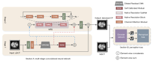
The denoising process we propose is not to directly remove the noise in LDCT but to gradually synthesize an image close to NDCT through a progressive MSCNN. The first stage of our proposal was to extract feature information from LDCT images, then refine the extracted features through the SCM, and pass them to the next stage. During the second stage, we introduced channel attention subnets, modelled the dependencies of each channel to improve the network’s presentation capabilities, and adjusted the features channel by channel, retaining the detail-rich features. In addition, based on the VGG perception loss, a self-encoding perception loss was also proposed to optimize the denoising model. Next, we detailed the network structure of the algorithm and the innovative modules presented in the network structure.

Network structure

The aim of LDCT image denoising is to generate CT images with better quality, less noise, and precise texture details. To achieve this goal, we must design a successful network structure. The overall process of the multistage network architecture is shown in Figure 1. Section A is composed of 2-stage sub-networks. The first stage is based on the dilated residual CNN sub-network, which uses LDCT images as input. The subnetwork learns rich context information in the receptive field and performs initial denoising on the input LDCT image. Since image denoising is a position-sensitive task, it requires pixel-to-pixel correspondence from input to output. Therefore, the second stage of the subnetwork concatenated the original LDCT image features and the image after the initial denoising characteristic and introduced the channel attention subnet. It is hoped that the dependency of each channel can be modelled to improve the network’s presentation ability, and the features can be adjusted channel by channel to preserve the detail-rich features. It is worth noting that instead of simply cascading sub-networks in multiple stages, we added a SCM between the 2 stages, establishing long-range spatial and inter-channel correlations to avoid useless information interference while generating more differentiated feature representations. In Section B, we used the NDCT image and the denoised CT image as input. The encoder network of the autoencoder trained by the self-supervised method learns compression coding features, which are used as the perceptual loss of the entire network structure.

Figure 1 Flowchart of MSCNN network: the first stage uses dilated residual convolution to extract multiscale context features and perform initial denoising, the second stage of the subnetwork concatenated the original LDCT image features and the image after the initial denoising characteristic and introduced the channel attention subnet. A supervised self-calibration module is added between the 2 stages, which learns to refine the features of one stage before passing it to the next stage. The pink and blue dotted arrows indicate the cross-level feature fusion mechanism. MSCNN, multistage convolutional neural network; LDCT, low-dose computed tomography.

Dilated residual convolutional neural network (DRCNN)

Under normal circumstances, the classic method of increasing the receptive field includes adopting a pooling layer in the network structure to perform the down-sampling process, design a larger filter, and stack more convolutional layers. Although the downsampling process using the pooling layer is widely used in classification tasks and has achieved good results, it is not recommended to use the pooling layer in the field of natural image super-resolution and medical image denoising. The main reason is that using the pooling layer to perform the downsampling process will result in the loss of structural details, which are essential for medical images. Even if the corresponding upsampling method (such as transposed convolution) is applied, these structural details cannot be wholly restored. Designing a larger filter and stacking more convolutional layers will consume memory resources and reduce the algorithm’s efficiency. Dilated convolution can achieve the purpose of rapidly increasing the receptive field by using only a tiny part of the network weight. We generally define one-dimensional (1D) dilated convolution based on the following mathematical Eq. [2]:

y(i)=∑k=1fx(i+r,k)ω(k)[2]

where x(i) represents the input of dilated convolution, and y(i) represents the output of dilated convolution. ω represents the weight vector of the filter with length f, and r represents the expansion rate.

The receptive field of the L-th convolution with a filter f×f and an expansion rate ofr can be expressed through the following mathematical Eq. [3]:

RFL=RFL−1+(f−1)r[3]

The total number of weights required by the N-layer convolutional network with a filter of f×f can be expressed through the following Eq. [4]:

MWeight=n×f2×c+n2×f2×(N−2)+n×f2×c[4]

among them, n represents the number of filters in each convolution layer, and c represents the convolutional channels. Table 1 lists the number of convolutional layers, the number of weights required to obtain the same receptive field under the same filter, and the input and output channels. The comparative results show that the dilated convolution can obtain a larger receptive field with only a small number of layers and weights.

To better demonstrate the denoising performance of dilated convolution, we designed a CNN with asymmetric dilation rate as a module of the entire LDCT denoising network structure. To obtain more image features, we added identity mapping to the output of the shallow convolution and the input of the deep convolution to optimize the entire network’s performance. The overall structure is shown in Figure 2. The network structure contains 7 convolutional layers with symmetric expansion rates, and the expansion rates are set to 1, 2, 3, 4, 3, 2, and 1. When the expansion ratio is set to 1, the expansion convolution is equivalent to ordinary convolution. The convolution kernel of each convolution layer is 3×3, and the filters in the first to sixth convolution layers are 64; the last layer of the convolution filter is set to 1. The batch normalization layer was added after the second to sixth layer convolution. The activation functions are all Leaky Rectified Linear Unit (LeakyReLU), and the step size in all convolution layers is set to 1. In this paper, to fully use the input image’s detailed information, we added an asymmetrical residual structure to improve the network’s performance. As shown inFigure 2, the output images of the first, second, and third layers are the same as those of the first layer. The input images of the fifth, sixth, and seventh layers are connected. These skip connections transfer the CT image’s low-level features to high-level ones, mainly since the initial input image contains many features (grey features, texture features, and shape features).

Figure 2 Schematic diagram of the proposed DRCNN architecture. DRCNN, dilated residual convolution neural network.

Attention mechanism

Attention mechanism can refine the perceptual information while retaining the context information and has been successfully applied to advanced tasks such as image classification (36,37), segmentation (38,39), and detection (37,40). In recent years, image denoise (41,42), ultra-resolution (43,44), image deblur (45,46), and other low-level tasks have also shown excellent results. Among them, the self-attention network can fully demonstrate the global dependency of each word (47) or image (40) in a sentence using multiplication between matrices. Squeeze and excitation networks can capture dependencies between channels by compressing global spatial information into channel descriptors (36). Zhang et al. (43) proposed a residual in the network, which focuses on learning high-frequency information through jump connections and adjusts channel characteristics adaptively, considering the dependence between channels. Zamir et al. (35), under the supervision and prediction of local ground truth, generated attention graphs to suppress the characteristics of less information. Under the weight of channel attention, the details of the original image were retained, indicating the effectiveness of the attention mechanism in image restoration. Song et al. (48) put forward multiple self-similar networks, using the relationship between non-local features and explained the effectiveness of the attention mechanism in CT image denoising tasks. Therefore, this section proposes 2 different types of attention structures embedded in the network structure we offer.

SCM

When we added the SCM module, we focused on improving CNN’s basic convolutional feature conversion process without adjusting the entire network model architecture, thereby enhancing the expression of the output features. We split a standard convolution into 4 small convolutions, adaptively establishing long-range spatial and inter-channel correlations around each point at each spatial location without increasing the amount of computation, while somewhat avoiding interference with some useless information about unrelated areas of global information, so that it can explicitly combine richer information to help CNN generate more differentiated representations.

As shown in Figure 3, first divided the input x∈R^C×H×W evenly along the channel direction to obtain 2 identical mappings x1,x2∈RC2×H×W. The dimension of the convolution kernel K is C×C×H×W, K was split into 4 small convolution kernels, each with different functions, which are respectively denoted as K₁, K₂, K₃, and K₄. Their dimensions were all C2×C2×H×W, and the size was 3×3. On the first path, we used K₂, K₃, and K₄ to self-calibrate x₁ and to obtain the output Y₁. To effectively collect each spatial location’s rich context information, convolution feature conversion was performed in 2 different scale spaces: the feature map in the original scale space and the downsampled latent space with smaller resolution (used for self-calibration). Considering that the downsampling part had a larger receptive field, we used the feature map in the latent space to transform the feature information to guide the feature transformation of the original feature space step by step. In the second path, we used K₁ to perform a simple convolution operation on x₂ to preserve the original spatial information and obtain the output result Y₁. Finally, the 2 path results Y₁ and Y₂ were connected in series to achieve the final output Y. The specific calculation process is as follows:

Fdown=AvgPoolr(x1)[5]

Y1=φ4{φ3(x1)⋅σ[Fup(φ2(Fdown))+x1]}[6]

Y2=φ1(x2)[7]

Figure 3 Schematic diagram of the proposed SCM. SCM, self-calibration module.

among them, φ₁, φ₂, φ₃, and φ₄ respectively represent 4 convolution operations, F_down refers to the downsampling process, this process mainly for the average pooling operation on the input x₁, where the filter is 4×4, the stride size is 4, and the r size is 4. The F_up describes the upsampling process and performs bilinear interpolation on the downsampling result, and σ is the sigmoid function.

Channel attention module (CAM)

Traditional CNN-based approaches often treat feature diagrams equally across channels, resulting in a lack of rational use of advanced and low-level feature information. To make full use of the characteristic information of each channel, we adopted the channel attention mechanism, with the aim of improving the network’s presentation ability by modelling the dependence of each channel and adjusting the features channel by channel, while retaining detailed features.

We introduced the native resolution subnet (NRS) in the second stage in Figure 1. The subnet contains multiple native resolution blocks (NRB); each NRB contains multiple CAMs. As shown in Figure 4, assuming that the input of the CAM is an H×W image, and the number of channels is C, to obtain the weight vector of the channel, a global average pooling operation was adopted for the input information. After pooling, 2 1×1 convolutional layers were first used to compress the channels, and then they were restored to fuse the information between the channels. Finally, the 1×1×C vector was converted into a weight vector through the sigmoid function. This process can be described through the following equation:

s=f(Fupδ(FdownG(z)))[8]

Figure 4 Diagram of the CAM in the proposed NRS in the second stage in Figure 1. CAM, channel attention module; NRS, native resolution subnet.

where z represents input data, G represents global average pooling, F_down represents the channel with a convolution layer of 1×1 downsampling operation, F_up represents the channel with a convolution layer of 1×1 upsampling operation, δ represents the Parametric Rectified Linear Unit (PReLU), and f represents the sigmoid activation function.

Objective function

Perceptual loss of autoencoding training

In previous work (33), the most commonly used perceptual loss for studying the structure of image denoising network has been several convolutional layers of VGG-19, neural training on the raw image data set ImageNet (https://image-net.org/), and the output of the 16th convolutional layer, which is as follows:

LVGG(G)=E(x,z)[1whd‖VGG(G(z))−VGG(x)‖F2][9]

where VGG() represents the feature map obtained from the VGG network, G(z) represents the denoising result of the LDCT image, x represents the NDCT image, and w, h, and d represent the width, height, and depth of the feature map, respectively.

Since CT images are usually a mixture of geometric shapes, textures, and non-uniformly distributed noise, the feature extraction of CT images is more complex and challenging than that of natural images. A potential problem of using VGG loss is that the VGG feature extractor is trained for natural image classification. If the transfer learns CT images, it often generates features unrelated to CT image denoising and even loses important details (34). Therefore, VGG loss is not the best perceptual loss function for LDCT denoising. However, the main challenge of training perceptual networks in specific domains is that CT datasets are usually unlabeled, making it impossible to apply supervised learning to train new neural networks from scratch or transfer existing DL models.

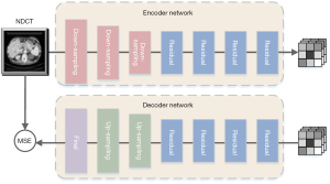
We designed a self-encoder network consisting of encoder networks and a decoder network to solve this complex problem. The network from the input CT images of normal dose can be processed through the encoder to learn compression coding. Then, it is reconstructed into the original input image through the decoder, and the whole training process is carried out in a self-supervised training method. The perceptual loss used in section B of Figure 1 only uses the encoder part of our autoencoder network. The decoder part is only used to train the entire autoencoder network. In the next section, we introduce the various components of the autoencoder network in detail.

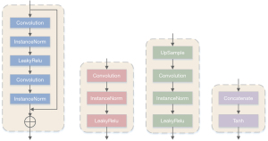
As shown in Figure 5, four different types of blocks: the residual block, the downsampling block, the upsampling block, and the final block are the autoencoder network’s core blocks. The downsampling block (Figure 4B) uses stride-size convolution to reduce the feature map’s dimensionality to obtain better computational efficiency. Compared with the max-pooling layer, stride-size convolution selects features for downsampling. The residual block (Figure 4A) contains residual connections, which integrate low-dimensional features into the calculation process of high-dimensional features. This design shows better performance for deep neural networks. The upsampling module (Figure 4C) converts the feature map to its original dimensions to generate the final output. We used the nearest neighbor interpolation upsampling layer and then used a convolutional layer for upsampling. We chose this design to replace the deconvolution layer to avoid the ‘checkerboard’ effect. The padding of all convolutional layers in the encoder and decoder blocks was reflection padding. By using this approach, better results can be provided at the edges of the generated image.

Figure 5 Basic building blocks of encoder and decoder: (A) residual block, (B) downsampling block, (C) upsampling block, and (D) final block.

The detailed content of the self-encoder network is shown in Figure 6. The encoder network contains 3 down-sampling blocks and 4 residual blocks, with 64, 128, 256, 256, 256, 256, and 256 filters, respectively. The decoder network contains 4 residual blocks, 2 upsampling blocks, and a final block, where the filters are 256, 256, 256, 256, 128, 64, and 1, respectively. The convolution kernel, step size, and padding number of the first downsampling block in the encoder are 7, 1, and 3, respectively. The convolution kernel, step size, and padding number of the second and third downsampling blocks are 4, 2, and 1. The residual block’s convolution kernel, step size, and padding number are all 3, 1, and 1. The decoder’s upsampling block’s convolution kernel, step size, and padding number are 5, 1, and 2, respectively. The final block’s convolution kernel, step size, and padding number are 7, 1, and 3, respectively. The autoencoder network uses the MSE objective function to constrain the original input image and the generated image.

Figure 6 Proposed autoencoder network; the pink module represents the downsampling block, the blue module represents the residual block, the green module represents the upsampling block, and the purple module represents the final block. NDCT, normal-dose computed tomography.

After the self-encoder network training was completed, we extracted the output of the encoder part as the learned feature and applied it to the perceptual loss function:

LAE(G)=E(x,z)[1whd‖ϕ(G(z))−ϕ(x)‖F2][10]

where Φ represents the encoder part of the self-encoding network, G(z) represents the denoising result of the LDCT image, x represents the NDCT image, and w, h, and d represent the width, height, and depth of the feature map, respectively.

Loss of structural restoration

Generally, in the field of image denoising, the most commonly used indicators to evaluate image quality are PSNR and structural similarity index measure (SSIM) (49). The higher the scores of these 2 indicators, the better the denoising effect and the richer the detailed information retained. Therefore, to improve the PSNR value, we compared the L₁ and L₂ loss functions more fully. The L₁ loss function, also called the mean absolute error (MAE) (50), and the L₂ loss, also called the MSE loss (51), are both based on the pixel average measurement method but have different effects in denoising. The L₂ loss focuses on penalizing relatively enormous pixel differences and tolerates relatively minor pixel differences. Based on this, in our denoising network, we used the L₁ loss function and expressed it through the following mathematical formula:

L1(G)=1N∑i=1N‖G(z)−x‖1[11]

where N represents the number of pixels, G(z) represents the denoising result of the LDCT image, and x represents the NDCT image.

Medical CT images of different dose levels have a strong feature correlation. The SSIM considers the perceived quality and texture information of the image from brightness and contrast. In the process of medical diagnosis, the SSIM is more in line with human visual observation than PSNR and MSE. Therefore, we introduced the classic SSIM and defined it according to the following formula:

SSIM(x,y)=2μxμy+c1μx2+μy2+c1⋅2σxy+c2σx2+σy2+c2[12]

where µ represents the average value of the 2 images compared, and σ represents the 2 images’ standard deviation. The C₁=(K₁L)² and C₂=(K₂L)² formulae are constants to eliminate numerical singularities, where L represents the maximum pixel value of the image, and k₁ and k₂ are constants. To obtain richer detailed structure and texture information in the image, we anticipated that the larger the value of SSIM, the better. In many cases, the gradient descent method was used to minimize the parameters. Therefore, we re-expressed the SSIM loss function using the following formula:

LSSIM(x,y)=1N∑i=1N1−SSIM(xi,yi)[13]

If only the L₁ loss is used in the structural restoration loss, the generated denoised image will be too smooth; similarly, if just the SSIM-based loss is used, the overall denoising effect will also be unsatisfactory. To balance noise reduction and structure maintenance, we combined 2 loss functions and gave them different weights. Finally, the structure recovery loss was expressed according to the following mathematical formula:

LSR=μL1+(1−μ)LSSIM[14]

Total loss function

We combined the different loss items introduced above into a mixed loss function to guide our entire denoising network. Our overall loss function includes the perceptual loss and structure recovery loss of self-encoding training. The general objective function formula is defined as follows:

Ltotal=LAE+λ1LSR[15]

Results

In this section, we verify the effectiveness of our proposed algorithm through experiments. First, we introduced the data set used in the experiment and the parameter settings required for the training process. Secondly, we performed ablation experiments on each module of the network structure to verify its effectiveness. Finally, we carried out the method proposed by ourselves and the most advanced method. The comparison verified the effectiveness of our overall network structure.

Experimental datasets

The primary purpose of our proposed network structure is to denoise LDCT. Therefore, our datasets used an actual clinical data set provided by the Mayo Clinic (Rochester, MN, USA). The image data of this dataset is made of the American Association of Physicists in Medicine (AAPM) LDCT game held in 2016. It contains 2,378 pairs of quarter- and normal-dose abdominal CT images of 10 patients. Our experiment divided the data set into 2 experimental parts. We trained and validated 8 patients and tested the remaining 2 patients.

We chose the simulated quarter-dose CT image for practical training in the training phase and the NDCT image was used as the training target value. Considering the limited number of CT images that could meet the requirements of our experiment, we also adopted the overlapping patch strategy, which not only finds spatial interconnection between patches but also significantly accelerates the convergence of the learning model (52). In terms of data preprocessing, the original LDCT and NDCT images were 512×512 pixels; we randomly divided the entire CT image into 20 overlapping 64×64 images of patches, resulting in 36,480 pairs of patches. The test set was a full-size image from both cases. To prevent overfitting caused by the complexity of the model, we took the “5-fold cross-validation” to train the network, and the data set was randomly divided into 5 copies, each training selected one of the data sets as a validation set, the remainder of the data set as a training set. To maintain rigor, in subsequent benchmark experiments, we used the same number of image patches for training. The parameter settings of the training process followed the parameter values mentioned in the original text for the entire experimental procedure. As shown in Figure 7, the CT Hounsfield unit (HU) scale was normalized, and their pixels value was scaled between 0 and 1 as the input to the network.

Figure 7 Scales of the CT HU are normalized, and their pixel values are normalized to [0, 1]. CT, computed tomography; HU, Hounsfield unit.

Parameter setting

The MSCNN network uses the adaptive moment estimation (ADAM) (53) optimizer training. The hyperparameter selection learning rate of the ADAM optimizer is α=1.0×e⁻⁴, and the exponential decay rates are settings β₁=0.9 and β₂=0.999. We set the learning rate of all convolutional layers in the network to 3×10⁻⁴, attenuated 0.5% after each epoch, and set the total epochs to 60.

Parameter selection plays a vitally important role in the performance of the algorithm. For the 2 hyperparameters λ and µ involved in the objective function, this paper reports experiments on the Mayo data set. First, the parameter values reported in the literature (50) were used as the references, and the values of λ and µ were adjusted to train the network. The test results’ average PSNR and SSIM values vary with the values of λ and µ, as shown in Table 2. It can be seen from the table that with the increase of λ and µ, the PSNR and SSIM values increase first and then decrease once λ=10 and µ=0.84 are reached, so that the test results achieve the best average PSNR and SSIM values. Therefore, the parameters were set to λ=10 and µ=0.84 in this experiment.

The second stage NRS in the network contains three NRBs, and each NRB uses 8 CABs. The proposed algorithm is written in Python on the Pytorch platform and implemented on an Intel Xeon Silver 4210R central processing unit (CPU), 64 GB RAM (Intel, Santa Clara, CA, USA), and 2 GPU cards (NVIDIA RTX A5000, NVIDIA, Santa Clara, CA, USA) with 48 GB memory to speed up the training process, which lasts for 10 h.

Ablation study of proposed methods

We conducted ablation experiments on each key module of the proposed network structure to verify each module’s performance.

Different loss functions lead to different denoising results

Previous studies have proposed various valuable and classic loss functions to study the mapping between low- and high-dose CT images. Therefore, this article also discusses the influence of different loss functions on the denoising effect. We discussed other loss functions on the denoising effect: L₁, L_SSIM, L_VGG, and L_AE. To show the effectiveness of the autoencoding perceptual loss, we verified the effectiveness of the loss under the CNN network architecture and the MSCNN network architecture. For the CNN network architecture, we combined the CNN network CNN-L_AE with autoencoding perceptual loss proposed in this article, CNN-L₁ with L₁ loss, CNN-L_SSIM with L_SSIM loss, and the CNN network with VGG perceptual loss CNN-L_VGG was the comparator. We compared MSCNN-L_AE with the autoencoding perceptual loss for the MSCNN network architecture, MSCNN-L₁ with L₁ loss, MSCNN-L_SSIM with L_SSIM loss, and MSCNN-L_VGG with VGG perceptual loss. We experimented with different network structures and compared the relationship between convergence and epoch.

The relationship between the average loss value of all the above neural networks and the epoch during the training process and measured by L₁ loss and VGG loss is shown in Figure 8. In Figure 8A, the relationship between the average L₁ loss value and 8 different network structures epochs is shown. Our proposed MSCNN-L_AE network is better than other networks based on MSCNN, but also MSCNN’s network converges faster and achieves the lower average L₁ loss value. Since the pure CNN structure is relatively simple, all CNNs that have not undergone multistage training can converge quickly. The CNN-L₁ uses L₁ loss as the objective function; CNN-L₁ obtains the lowest error value in the L₁ loss metric. The entire convergence curve decreases speedily and then converges smoothly, and the convergence speed is also the fastest. However, the excessive smoothness of the whole CNN-L₁ convergence curve is problematic. The convergence curve of CNN-L_SSIM shows a trend of first declining and then rising. The MSCNN-L_SSIM also shows a similar floating trend with CNN-L_SSIM in terms of L₁. This shows that the L_SSIM-based method and the mean-based method have different emphases in minimizing the perceptual similarity between the real and the generated NDCT image.

Figure 8 Relationship between the convergence of different network structures and epoch: (A) L₁ loss convergence; (B) VGG loss convergence. VGG, visual geometry group; CNN-L₁, convolution neural network with L₁ loss; CNN-L_SSIM, convolution neural network with L_SSIM loss; CNN-L_VGG, convolution neural network with L_VGG loss; CNN-L_AE, convolution neural network with L_AE loss; MSCNN-L₁, multistage convolution neural network with L₁ loss; MSCNN-L_SSIM, multistage convolution neural network with L_SSIM loss; MSCNN-L_VGG, multistage convolution neural network with L_VGG loss; MSCNN-L_AE, multistage convolution neural network with L_AE loss.

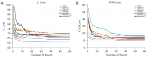
The relationship between the VGG loss and 8 different network structures epochs is shown in Figure 8B. We documented that our proposed MSCNN-L_AE network has the fastest convergence speed by comparing the MSCNN-based network. The VGG loss of MSCNN-L_AE is very close to the VGG loss of MSCNN-L_VGG, and MSCNN-L_VGG obtains a lower VGG loss value mainly because the MSCNN-L_VGG network takes VGG loss as its objective function. The CNN-L_VGG takes VGG loss as the inherent training objective function; CNN-L_VGG has the fastest convergence speed in VGG loss measurement and the lowest loss value. However, a lower VGG loss value does not mean that the algorithm has received a better denoising effect. Subsequent experimental results showed that the noise generated by the VGG-based network structure will weaken its advantages. Moreover, Table 3 also provides a comparison of the quantitative effects of different loss functions. By comparing CNN-L_VGG and CNN-L_AE, the self-encoding perceptual loss further improves the PSNR and SSIM. In the comparison of results based on the multistage network architecture, similar results were also obtained, supporting the effectiveness of the self-encoding perceptual loss in the network structure.

Effectiveness of DRCNN

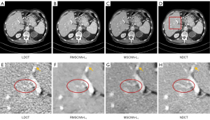
To verify the effectiveness of the DRCNN in the network structure, we replaced the DRCNN in MSCNN with regular CNN, compared it with MSCNN, and labelled them as RMSCNN-L₁ and MSCNN-L₁ for convenience. As shown in Figure 9—the first rows of Figure 9B,9C—the denoised image of RMSCNN-L₁ is too smooth, and there are more structural distortions. In the region of interest (ROI) area indicated by the enlarged rectangular frame, it can be observed that the CNN-based method has jagged marks on the boundary of the white area indicated by the yellow arrow. Our proposed MSCNN-L₁ is more effective in maintaining edge features. As shown in the red ellipses in Figure 9F,9G, RMSCNN-L₁ blurs the overall structure details and causes part of the structure to be lost; in contrast, our MSCNN-L₁ method restored the details better. Table 3 also shows the quantitative results of denoising. The results show that the PSNR and SSIM of MSCNN-L₁ are superior to RMSCNN-L₁.

Figure 9 Comparison of the denoising CT images generated by the RMSCNN-L₁ and the MSCNN-L₁: (A) LDCT image, (B) denoised image generated by the RMSCNN-L₁, (C) denoised image generated by the MSCNN-L₁, (D) NDCT image, (E) ROI of LDCT image, (F) ROI of RMSCNN-L₁, (G) ROI of MSCNN-L₁, and (H) ROI of NDCT. The red rectangle and the red ellipse represent the reconstruction area we are concerned with. The yellow arrow represents the structural recovery area of concern. CT, computed tomography; RMSCNN-L₁, multistage convolution neural network based on the regular convolution neural network with L₁ loss; MSCNN-L₁, multistage convolution neural network with L₁ loss; LDCT, low-dose CT image; NDCT, normal dose CT image; ROI, region of interest.

Effectiveness of the SCM

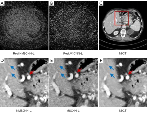
The SCM is an attention mechanism. To demonstrate the importance of SCM, we compared MSCNN with the MSCNN network framework without SCM, as shown in Figure 10. These network structures are trained through L₁ loss, and they are labelled NMSCNN-L₁ and MSCNN-L₁, respectively. The ROI area of the denoised effect of 2 network structures is shown in Figure 10D,10E. Comparing the location indicated by the blue arrow with NMSCNN-L₁ without a SCM, MSCNN-L₁ avoids some waxy artefacts and makes the organ surface look smoother. By comparing the area indicated by the red arrow, MSCNN-L₁ also produces a sharper edge structure than NMSCNN-L₁ without a SCM. The residual effect is shown in Figure 10A,10B, where it can be observed that the SCM we proposed avoids more noise, indicating that the denoised image generated by the MSCNN-L₁ network is closer to the NDCT image. Furthermore, Table 3 also gives the quantitative results of denoising, and the results show that the PSNR and SSIM of MSCNN-L₁ are better than NMSCNN-L₁. We verified the importance of the SCM in CT imaging through ablation experiments.

Figure 10 Comparison of denoising CT images produced by NMSCNN-L₁ and MSCNN-L₁: (A) Resi.NMSCNN-L₁ denoising image, (B) Resi.MSCNN-L₁ denoising image, (C) NDCT image, (D) ROI of NMSCNN-L₁, (E) ROI of MSCNN-L₁, and (F) ROI of NDCT. The red rectangle represents the area of image reconstruction we are interested in; blue and red arrows are used to indicate image recovery details. CT, computed tomography; NMSCNN-L₁, multistage convolution neural network none of self-calibration module with L₁ loss; MSCNN-L₁, multistage convolution neural network with L₁ loss; Resi.NMSCNN-L₁, residual image between NDCT image and NMSCNN-L₁ denoising image; Resi.MSCNN-L₁, residual image between the NDCT image and the MSCNN-L₁ denoising image; NDCT, normal dose CT image; ROI, region of interest.

Effectiveness of multistage network structure

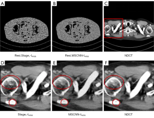
To verify the effectiveness of a multi-stage network, we compared multi-stage network MSCNN and single-stage network, as shown in Figure 11. As can be seen from Figure 11D,11E, the MSCNN-L_VGG network trained based on VGG perceptual loss eliminates more fringe artifacts and produces clearer and finer structural texture information. As shown in Figure 11A,11B, the denoised image generated by the MSCNN-L_VGG network is more explicit, which demonstrates that the denoised image generated by MSCNN-L_VGG is closer to the ground truth. The quantitative results in Table 3 also show that the MSCNN-L_VGG network achieved higher PSNR and SSIM than the Stage1-L_VGG network. We verified the importance of a multistage network structure in CT imaging through ablation experiments.

Figure 11 Comparison of the denoising CT image generated by Stage₁-LV_GG and MSCNN-L_VGG: (A) Resi.Stage₁-L_VGG denoising image, (B) Resi.MSCNN-L_VGG denoising image, (C) NDCT image, (D) ROI of Stage1-L_VGG, (E) ROI of MSCNN-L_VGG, and (F) ROI of NDCT. Red rectangles, red circles and red ellipses represent the areas of image reconstruction we are concerned with. CT, computed tomography; Stage₁-L_VGG, stage1 network structure in Figure 1 with visual geometry group loss; MSCNN-L_VGG, multistage convolution neural network with visual geometry group loss; Resi.Stage₁-L_VGG, residual image between the NDCT image and the Stage₁-L_VGG denoising image; Resi.MSCNN-L_VGG, residual image between NDCT image and MSCNN-L_VGG denoising image; NDCT, normal dose CT image; ROI, region of interest.

Effectiveness of self-encoding perceptual loss

To verify our proposed self-encoding perceptual loss effectiveness, we visualized the feature map between the self-encoder and the traditional ImageNet trained VGG. For VGG, we used the VGG-19 network. Its architecture contains 16 convolutional layers and 3 fully connected layers. We chose the output of the 16th layer as the extracted features. For our proposed self-supervised autoencoder, we selected the output of the encoder part as the extracted feature. We extracted 64 feature maps with the same spatial size as the input for the 2 methods and compared them visually, as shown in Figure 12. The qualitative result graph shows that the feature map extracted by the self-encoding network is more evident in contour and texture than the feature map extracted by the VGG network. At the same time, in Table 3, the quantitative comparison results of CNN-L_VGG, CNN-L_AE, MSCNN-L_VGG, and MSCNN-L_AE are also presented, proving the effectiveness of self-encoding perceptual loss in the network structure.

Figure 12 Schematic diagram of the feature map generation process based on the VGG and self-encoding networks: the top row is the input image, the middle is the VGG network and the self-encoding network, the bottom is the feature map extracted from the image, the left column of the bottom row is the feature map extracted by the VGG network, and the right column is the feature map extracted by the self-encoding network. VGG, visual geometry group.

Qualitative comparison of denoising results

We selected 2 patients’ CT images from the test set, and their denoising effects were described in detail, including some anatomical information of the lesion structure. To show the performance of the algorithm, we not only compared the traditional classic denoising algorithm block-matching and 3D filtering (BM3D) (54) but also compared several latest denoising algorithms, including the CNN-based network structure RED-CNN (26), GAN-based network structure Wasserstein generative adversarial network with visual geometry group perceptual loss (WGAN-VGG) (27), least squares generative adversarial network with a hybrid loss function (LSGAN-L_Hybrid) (29), cycle-consistent generative adversarial network with attention (CAGAN) (32), and dilated residual learning (DRL) based on cascade network (33). The qualitative comparison results of 2 abdominal CT images are shown in Figure 13 and Figure 15. To more clearly evaluate the image denoising effect of different denoising network models, we also marked the ROI in the resulting image. This area was enlarged and compared, as shown in Figures 14,16, respectively. It is worth noting that all models’ denoising tasks were focused on image content restoration and image denoising.

Figure 13 Results of abdominal CT scans from the test set using different methods: (A) LDCT, (B) BM3D, (C) RED-CNN, (D) WGAN-VGG, (E) LSGAN-L_Hybrid, (F) DRL, (G) CAGAN, (H) MSCNN, and (I) NDCT, the red rectangular frame represents the enlarged area of Figure 14. CT, computed tomography; LDCT, low-dose CT; BM3D, block-matching and 3D filtering; RED-CNN, residual encoder-decoder convolutional neural network with L₂ loss; WGAN-VGG, Wasserstein generative adversarial network with visual geometry group perceptual loss; LSGAN-L_Hybrid, least squares generative adversarial network with a hybrid loss function; DRL, dilated residual learning; CAGAN, cycle-consistent generative adversarial network with attention; MSCNN, multistage convolution neural network; NDCT, normal-dose CT image.

Figure 15 Results of abdominal CT scans from the test set using different methods: (A) LDCT, (B) BM3D, (C) RED-CNN, (D) WGAN-VGG, (E) LSGAN-L_Hybrid, (F) DRL, (G) CAGAN, (H) MSCNN, and (I) NDCT, the red rectangular frame represents the enlarged area of Figure 16. CT, computed tomography; LDCT, low-dose CT; BM3D, block-matching and 3D filtering; RED-CNN, residual encoder-decoder convolutional neural network with L₂ loss; WGAN-VGG, Wasserstein generative adversarial network with visual geometry group perceptual loss; LSGAN-L_Hybrid, least squares generative adversarial network with a hybrid loss function; DRL, dilated residual learning; CAGAN, cycle-consistent generative adversarial network with attention; MSCNN, multistage convolution neural network; NDCT, normal-dose CT image.

Figure 14 Enlarged part of the ROI marked by the red rectangle in Figure 13. (A) LDCT, (B) BM3D, (C) RED-CNN, (D) WGAN-VGG, (E) LSGAN-L_Hybrid, (F) DRL, (G) CAGAN, (H) MSCNN, and (I) NDCT, the red circle indicates structural deformation, and the green and blue arrows indicate two organizational structures. LDCT, low-dose computed tomography; BM3D, block-matching and 3D filtering; RED-CNN, residual encoder-decoder convolutional neural network with L2 loss; WGAN-VGG, Wasserstein generative adversarial network with visual geometry group perceptual loss; LSGAN-L_Hybrid, leasts squares generative adversarial network with a hybrid loss function; DRL, dilated residual learning; CAGAN, cycle-consistent generative adversarial network with attention; MSCNN, multistage convolution neural network; NDCT, normal-dose CT image; ROI, region of interest.

Figure 16 Enlarged part of the ROI marked by the red rectangle in Figure 15: (A) LDCT, (B) BM3D, (C) RED-CNN, (D) WGAN-VGG, (E) LSGAN-L_Hybrid, (F) DRL, (G) CAGAN, (H) MSCNN, and (I) NDCT. The red arrow indicates structural deformation. LDCT, low-dose computed tomography; BM3D, block-matching and 3D filtering; RED-CNN, residual encoder-decoder convolutional neural network with L₂ loss; WGAN-VGG, Wasserstein generative adversarial network with visual geometry group perceptual loss; LSGAN-L_Hybrid, least squares generative adversarial network with a hybrid loss function; DRL, dilated residual learning; CAGAN, cycle-consistent generative adversarial network with attention; MSCNN, multistage convolution neural network; NDCT, normal-dose CT image; ROI, region of interest.

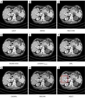
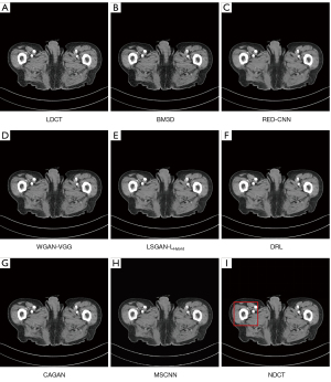
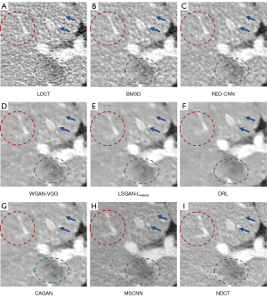
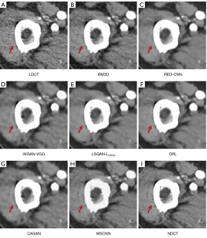
The LDCT image and the corresponding NDCT image are shown in Figure 13A,13H, which clearly display the substantial image differences. The red rectangle in Figure 13H marks the lesion and/or metastasis in the image. The red rectangular area in Figure 15H shows low-density liver lesions. In the ROI area of NDCT shown in Figures 14H,16H, these lesions can be observed; contrastingly, as can be seen in Figures 14A,16A, compared with NDCT, the initial LDCT image is severely degraded, and the critical structural features for clinical diagnosis are blurred. All the network structures in the figure show different degrees of denoising effects. Although the BM3D algorithm suppresses the noise to a certain extent, in denoised images Figures 13B,15B can be seen, some block and grid artifacts are present in the entire denoised image, and some edges and small structures are blurred. The RED-CNN method is a denoising method based on the mean value. The process is based on the mean value and can effectively remove noise, but its shortcoming is that it easily blurs the reconstructed image. It can be observed from Figure 13C that although RED-CNN significantly suppresses more noise, it obscures much essential structural information in the hilar area. In the enlarged ROI of Figures 14C,16C, although RED-CNN can make the image look less noisy, it transitions and obfuscates some anatomical structure information. There is a big gap in the precision of RED-CNN compared with the original NDCT.

In the advanced denoising method based on the GAN network, the images produced by the WGAN-VGG algorithm in Figures 13D,15D show better visual effects and structural detail preservation. However, the area near the red circle in Figure 14D and the red arrow in Figure 16D show that the algorithm may severely distort the structural information of the original image. The main reason is that because the VGG loss is based on a pretrained CNN network of ImageNet, the detailed features of natural images are entirely different from those of CT images. Although pixel-based measurement methods have good noise reduction performance, the content is blurred to a certain extent, resulting in the loss of structural details. The method based on perceptual loss can preserve texture and structure better than the method based on the mean value. Compared with WGAN-VGG, LSGAN-L_Hybrid, and CAGAN, as shown by the red circles in Figures 14,16, our proposed MSCNN can show portal vein metastasis more clearly and better preserve portal vein information.

In the cascade-based network, we compared the most advanced DRL algorithm. We know that Figures 13F,15F generated by the DRL algorithm are too smooth, the structure is not clear, and the texture is not apparent. A better visual effect in image details and more structural components similar to NDCT images in human perception evaluation is shown in Figure 15G. Based on a comparison of the positions indicated by the 2 blue arrows in Figure 14F,14G. Figure 14F looks more or less blurred and sometimes even disappears, while Figure 14G remains visible. Compared with all the previous methods, the noise reduction advantage of the MSCNN method is undeniable, especially in the dark background area in the green ellipse in Figure 14B-14G. The 2 blue arrows in Figure 14B-14G indicate that some detailed structures are lost in all denoised images. These details are almost smoothed into the background area by all denoising methods, especially in BM3D, RED-CNN, and DRL; the MSCNN method yields the least detailed information. By comparing the low-density liver lesions in the CT image of the abdomen in Figure 16, although all methods have grey-black shadows, MSCNN has more conspicuous shadow areas, which are beneficial for disease diagnosis. In summary, our proposed MSCNN network achieves a better balance between noise reduction and structural protection, resulting in better image quality.

Quantitative analysis

To quantitatively analyze the reconstruction results of different algorithms, 3 objective evaluation indexes, namely PSNR, SSIM, and visual information fidelity (VIF), were used in this paper to evaluate the quality of denoising images quantitatively. The PSNR is an evaluation index for evaluating image quality based on the error between corresponding pixels. The greater the PSNR value, the greater the ratio between (I) the detailed information that needs to be retained and (II) the noise information that needs to be suppressed in the generated image; that is, the more complete the valuable information of the image is retained, the better the denoising effect of the generated image. The SSIM measures image similarity from 3 aspects: brightness, contrast, and structure. The more significant the SSIM value, the better the visual effect of the generated image. The VIF is a measure of the fidelity of an image’s visual information as defined by Sheikh et al. (55). The larger the VIF value, the better the quality of the generated image.

As shown in Figure 17, RED-CNN achieved higher PSNR and SSIM. Since the nature of the PSNR is to regress to the mean, the regression optimization algorithm based on the norm has a higher PSNR value than other feature-based models. However, although RED-CNN gets a good score on the image quality measurement, it can still visually evaluate the image content in the case of excessive smoothness. Therefore, these indicators may not be comprehensive enough to assess image quality and indicate diagnostic performance.

Figure 17 Comparison of quantitative results of image processing on the test set with different methods: the three metrics are PSNR, SSIM, and VIF. PSNR, peak signal-to-noise ratio; SSIM, structural similarity; VIF, visual information fidelity; LDCT, low-dose computed tomography; BM3D, block-matching and 3D filtering; RED-CNN, residual encoder-decoder CNN with L₂ loss; WGAN-VGG, Wasserstein generative adversarial network with convolutional neural network perceptual loss; LSGAN-L_Hybrid, least squares generative adversarial network with a hybrid loss function; DRL, dilated residual learning; CAGAN, cycle-consistent generative adversarial network with attention; MSCNN, multistage convolution neural network.

Although WGAN-VGG, LSGAN-L_Hybrid, and CAGAN obtain lower PSNR and SSIM values, they can provide better visual quality and better statistical properties. The low scores of WGAN-VGG, LSGAN-L_Hybrid, and CAGAN may be due to the loss of subtle structural information or noise features affecting diagnostic accuracy. The DRL also obtained higher PSNR and VIF scores due to the cascaded network-based and MSE loss effectiveness. Both PSNR and SSIM pay more attention to pixel-level similarity, and VIF uses natural statistical models to pay more attention to the characteristics of the human visual system. We conclude that MSCNN has obtained the best scores of all indicators compared with the above algorithm. The quantitative analysis results show that the MSCNN network architecture proposed in this paper can improve the denoising performance.

Visual assessments

To verify the algorithm’s effectiveness regarding clinical images, we invited 3 radiologists to evaluate 20 sets of images visually. These 20 groups of images were randomly selected from the data set. Each group of images included an LDCT image and 7 images generated by 7 different denoising algorithms. A corresponding NDCT image was used as the reference object. The 3 radiologists used 4 indicators, noise suppression (NS), artifact reduction (AR), detail restoration (DR), and comprehensive quality (CQ) to evaluate the image quality after denoising. The evaluation score ranged from 1 to 5 points, with 1 representing ‘bad’ and 5 representing ‘excellent’. Each radiologist independently evaluated the final score. The CQ score of each algorithm was the average score based on the 3 evaluation criteria. The final score was expressed as the average of the 3 radiologists’ scores and standard deviations. Table 4 lists the quantitative results of the final evaluation.

Consistent with our expectations, the LDCT images were severely damaged due to the decreased radiation dose, and their final evaluation score was the lowest. In this study, all denoising models improved their scores to a certain extent. In Table 4 we can observe that RED-CNN had the highest score on the NS index, but it lost more detailed information. This shows that methods based on the MSE loss function can generally obtain better noise reduction performance but are not good at detail recovery. The network based on perceptual loss achieved better scores in DR and artifact removal. The WGAN-VGG, CAGAN, and our proposed MSCNN network all maintained detailed information very well, but the noise reduction effect of the MSCNN network was better. This evaluation result also confirmed our experimental results. The MSCNN achieved the best balance between image noise reduction, improved perception quality, and structural DR with self-calibration and auto-encoding modules. It also had the best overall effect on diagnosis.

Discussion

This study’s primary purpose was to denoise LDCT images so that denoised CT images could get as close as possible to normal dose CT images. To this end, we introduced the multistage progressive network architecture proposed by Zamir et al. (35) into the LDCT imaging process. We designed a multistage, attention module-driven, end-to-end training-based network structure designed explicitly for CT imaging.

First of all, we carefully compared the natural image denoising method of the literature (35) with our LDCT denoising method, which can be explained as follows:

• First, the crucial difference between natural and medical images in the imaging process needs to be considered. Noise distributions in natural images are often modelled as mixed Poisson and Gaussian distributions, while noise distributions in CT imaging are closer to Poisson distributions. Natural images belong to multichannel color images, while medical images are single-channel grayscale images. The fine structure of background tissue with very high similarity in sequence CT images is vital for medical images, but more attention should be given to valuable ROI of natural images.
• For the input data of the network structure, we put forward an input strategy applicable to the CT image. Since CT images are single-channel grayscale images, the training database may not contain many valid images. One of the most common experimental strategies in LDCT noise removal tasks is to generate overlapping patches (32), which better represent the local characteristics of the image and increase the number of training samples (56). Considering the limited number of CT images that could meet the requirements of our experiment, we additionally adopted the overlapping patch strategy, which not only considers spatial interconnection between patches but also significantly accelerates the convergence of the learning model (52). In terms of data preprocessing, the original LDCT and NDCT images were 512×512 pixels, and our denoising model randomly divided the entire CT image into 20 overlapping 64×64 image patches for training.
• It has been proposed in the literature (35) that under the supervision and prediction of local ground truth, an attention graph be generated to suppress the characteristics of the current stage with less information, and that only valuable features be allowed to propagate to the next stage. On the basis of this, we added SCMs to improve CNNs’ basic convolutional feature conversion process without adjusting the entire network model architecture and to adaptively establish long-range spatial and inter-channel correlations around each point at each space location without increasing the amount of computation. Moreover, explicitly combining richer information can help CNNs to generate more differentiated representations. This type of structural design is mainly because of the high correlation between human tissues and medical images, and the important information is also included in the structure with fewer features. This leads to the ability to distinguish areas with fewer features and those with more features in the global information without introducing additional parameters and model complexity.
• Traditional CNN-based approaches often treat feature diagrams equally across channels and lack the rational use of advanced and low-level feature information. It has been reported (35) that several channel attention modules can be applied to the original image of the input, thus maintaining the fine details from the input image to the output image. We referred to this design and applied it in the LDCT denoising process by modelling the dependence of each channel to improve the network’s presentation ability and adjusting the features channel by channel, thus retaining the detail-rich features.
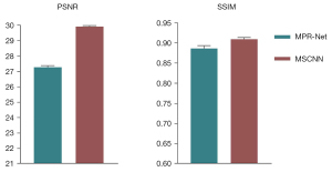
• To verify the validity of the proposed algorithm, we compared the network framework presented in the literature (35). In the course of experimental comparison, due to the differences between the natural and grayscale images, we improved the multistage progressive restoration network (MPR-Net) proposed in the literature (35). First, we changed the input convolution layer for the first, second, and third stages of the MPR-Net in the literature (35) to 1 for the input channel size. Second, we added a convolution layer of 1×1 before the output results of the first and second stages to guarantee that the output channel size was also 1. Finally, using the same experimental setup and training strategy, we trained and validated MPR-Net and our proposed MSCNN. Experimental comparisons were made on the test set, the qualitative results are shown in Figures 18,19Figure 20.
  

  Figure 18 Results of abdominal CT scans from the test set using different methods: (A) LDCT, (B) MPR-Net, (C) MSCNN, and (D) NDCT. CT, computed tomography; LDCT, low-dose CT; MPR-Net, multistage progressive restoration network; MSCNN, multistage convolution neural network; NDCT, normal-dose CT image.
  

  Figure 19 Results of abdominal CT scans from the test set using different methods: (A) LDCT, (B) MPR-Net, (C) MSCNN, and (D) NDCT. CT, computed tomography; LDCT, low-dose CT; MPR-Net, multistage progressive restoration network; MSCNN, multistage convolution neural network; NDCT, normal-dose CT image.
  

  Figure 20 Comparison of quantitative results of image processing on the test set with different methods: the 2 metrics are PSNR and SSIM. PSNR, the peak signal-to-noise ratio; SSIM, structural similarity; MPR-Net, multistage progressive restoration network; MSCNN, multistage convolution neural network.
• The qualitative comparison results of the 2 abdominal CT images are shown in Figures 18,19Figure 18A,18D, and there is a significant difference between the 2 image types. It can be observed from Figures 18B,19BFigures 18C,19CFigure 20 also show that MSCNN achieves high PSNR and SSIM values. The reason may be that the network structure and parameter settings of the MPR-Net algorithm are designed for natural images, the training process is more inclined to learn the characteristic information of natural images, and the experimental effect on grayscale images is not good.

As the CT images of the same site and homomorphism are very similar, and subtle changes in background tissue with very high similarity may represent lesions, all the information in a medical image, including small texture information, has a potential use. Our proposed MSCNN strikes a better balance between image noise reduction, improved perceived quality, and structural DR.

To verify the effectiveness of the proposed algorithm, we compared it with traditional denoising methods and DL denoising methods in recent years.

Since the noise in LDCT images is mainly Poisson noise, it is challenging to model non-uniformly distributed noise in the image domain accurately. However, BM3D (54) is suitable for specific noise distribution modelling methods, but is not ideal for CT image data. However, the DL method represented by a CNN has a strong knowledge expression ability and is suitable for various complex functions. In the qualitative and quantitative comparison of the experimental process, we also showed that the DL-based methods RED-CNN (26), WGAN-VGG (27), LSGAN-L_Hybrid (29), CAGAN (32), DRL (33), and our proposed MSCNN are superior to those based on the traditional denoising method BM3D. The DL-based methods show superior performance in removing noise and restoring details. Therefore, the conventional denoising method cannot achieve a better denoising effect compared with other DL denoising methods.

Both DRL (33) and our proposed MSCNN are based on multistage denoising methods. The primary purpose of the multistage denoising method is to gradually generate denoised images by progressively adopting a lighter subnetwork at each stage and decompose complex denoising tasks into simpler subtasks. Our experiments demonstrated that this design method is effective. Still, compared with our proposed MSCNN, because the DRL algorithm uses the same subnetwork at each stage, it has obtained suboptimal performance for each evaluation index.

The loss function has an important influence on the denoising process of LDCT images. When we only used the mean-based loss function for training, although we could obtain better PSNR and SSIM, in qualitative comparisons, the images generated by these methods are too smooth to satisfy the visual requirements of the human visual system. When we used the feature-based method for training, it retained more structural details than the mean-based method. However, the perceptual loss of pretraining VGG based on ImageNet may produce irrelevant features, resulting in content distortion. Therefore, we proposed the self-encoding perceptual loss based on VGG, combined the best characteristics of L₁ and SSIM, and used the hybrid loss function to optimize the image quality of LDCT.

Although our proposed method improves the denoising of LDCT images, it still has certain limitations. First, compared with the corresponding NDCT image, the generated image still contains subtle structural deformations, and some structural differences are not completely matched. In addition, medical images are usually 3D images, but we only studied 2D slices, ignoring the spatial information between slices. We plan to build a 3D model to fully utilize spatial information between different CT slices in future research. In addition, we will study the quality evaluation system and evaluation indicators specifically for CT images to evaluate CT images more rigorously.

Conclusions

Our work mainly proposes an end-to-end training-based CT image reconstruction algorithm. We suggest emphasizing the image’s details and restoring the LDCT image structure to improve diagnostic performance.

The main achievements of this paper were as follows: (I) We proposed a MSCNN architecture to suppress noise and preserve details. The first stage performs initial noise reduction on LDCT images. The second stage introduces the channel attention subnet and models the dependencies of the channel to the improved network’s presentation. Hereby, the features that cannot be adjusted channel by channel lead to the loss of detail-rich features. (II) A self-calibration mechanism was introduced between the 2 stages, with long-range spatial and inter-channel correlations to avoid using information and processing more than the selected features. (III) A self-supervised learning scheme was used to train the autoencoder network to solve the ill-posed problem of CT image feature extraction. Finally, experimental validation was carried out on the clinical dataset provided by the National Institutes of Health-American Association of Physics in Medicine-Mayo Challenge 2016. The results showed that the methods we proposed could effectively enhance the noise removal capability of traditional CNN and obtain better results.

In future research work, we intend to collect clinical data from several partner hospitals for experimental validation. Furthermore, we will also consider the design of different network structures based on the GAN architecture to evaluate its impact on radiological characteristics.

Acknowledgments

Funding: This work was partly supported by the National Natural Science Foundation of China (61872261), the Open Funding Project of the State Key Laboratory of Virtual Reality Technology and Systems, Beihang University (VRLAB2020B06), and received a Prevention and Control Research Project Grant of Shanxi Province (XE-2020-5-04).

Footnote

Reporting Checklist: The authors have completed the MDAR checklist. Available at https://dx.doi.org/10.21037/qims-21-465

Conflicts of Interest: All authors have completed the ICMJE uniform disclosure form (available at https://dx.doi.org/10.21037/qims-21-465). The authors have no conflicts of interest to declare.

Ethical Statement: The authors are accountable for all aspects of the work in ensuring that questions related to the accuracy or integrity of any part of the work are appropriately investigated and resolved. The study was conducted in accordance with the Declaration of Helsinki (as revised in 2013).

Open Access Statement: This is an Open Access article distributed in accordance with the Creative Commons Attribution-NonCommercial-NoDerivs 4.0 International License (CC BY-NC-ND 4.0), which permits the non-commercial replication and distribution of the article with the strict proviso that no changes or edits are made and the original work is properly cited (including links to both the formal publication through the relevant DOI and the license). See: https://creativecommons.org/licenses/by-nc-nd/4.0/.

References

1. Bencardino JT. Radiological Society of North America (RSNA) 2010 Annual Meeting. Skeletal Radiol 2011;40:1109-12. [Crossref] [PubMed]
2. Donya M, Radford M, ElGuindy A, Firmin D, Yacoub MH. Radiation in medicine: Origins, risks and aspirations. Glob Cardiol Sci Pract 2014;2014:437-48. [Crossref] [PubMed]
3. Ehman EC, Yu L, Manduca A, Hara AK, Shiung MM, Jondal D, Lake DS, Paden RG, Blezek DJ, Bruesewitz MR, McCollough CH, Hough DM, Fletcher JG. Methods for clinical evaluation of noise reduction techniques in abdominopelvic CT. Radiographics 2014;34:849-62. [Crossref] [PubMed]
4. Manduca A, Yu L, Trzasko JD, Khaylova N, Kofler JM, McCollough CM, Fletcher JG. Projection space denoising with bilateral filtering and CT noise modeling for dose reduction in CT. Med Phys 2009;36:4911-9. [Crossref] [PubMed]
5. Balda M, Hornegger J, Heismann B. Ray contribution masks for structure adaptive sinogram filtering. IEEE Trans Med Imaging 2012;31:1228-39. [Crossref] [PubMed]
6. Wang J, Li T, Lu H, Liang Z. Penalized weighted least-squares approach to sinogram noise reduction and image reconstruction for low-dose X-ray computed tomography. IEEE Trans Med Imaging 2006;25:1272-83. [Crossref] [PubMed]
7. Jing W, Lu H, Li T, Liang Z. Sinogram noise reduction for low-dose CT by statistics-based nonlinear filters. Proc. SPIE 5747, Medical Imaging 2005: Image Processing (29 April 2005). doi: 10.1117/12.595662.10.1117/12.595662
8. Niu T, Zhu L. Accelerated barrier optimization compressed sensing (ABOCS) reconstruction for cone-beam CT: phantom studies. Med Phys 2012;39:4588-98. [Crossref] [PubMed]
9. Bian Z, Ma J, Huang J, Zhang H, Niu S, Feng Q, Liang Z, Chen W SR-NLM. a sinogram restoration induced non-local means image filtering for low-dose computed tomography. Comput Med Imaging Graph 2013;37:293-303. [Crossref] [PubMed]
10. Shangguan H, Zhang Q, Liu Y, Cui X, Bai Y, Gui Z. Low-dose CT statistical iterative reconstruction via modified MRF regularization. Comput Methods Programs Biomed 2016;123:129-41. [Crossref] [PubMed]
11. Xu Q, Yu H, Mou X, Zhang L, Hsieh J, Wang G. Low-dose X-ray CT reconstruction via dictionary learning. IEEE Trans Med Imaging 2012;31:1682-97. [Crossref] [PubMed]
12. Adler J, Oktem O. Learned Primal-Dual Reconstruction. IEEE Trans Med Imaging 2018;37:1322-32. [Crossref] [PubMed]
13. Chen Z, Zhang Q, Zhou C, Zhang M, Yang Y, Liu X, Zheng H, Liang D, Hu Z. Low-dose CT reconstruction method based on prior information of normal-dose image. J Xray Sci Technol 2020;28:1091-111. [Crossref] [PubMed]
14. Li Z, Yu L, Trzasko JD, Lake DS, Blezek DJ, Fletcher JG, McCollough CH, Manduca A. Adaptive nonlocal means filtering based on local noise level for CT denoising. Med Phys 2014;41:011908. [Crossref] [PubMed]
15. Chen Y, Yin X, Shi L, Shu H, Luo L, Coatrieux JL, Toumoulin C. Improving abdomen tumor low-dose CT images using a fast dictionary learning based processing. Phys Med Biol 2013;58:5803-20. [Crossref] [PubMed]
16. Sheng K, Gou S, Wu J, Qi SX. Denoised and texture enhanced MVCT to improve soft tissue conspicuity. Med Phys 2014;41:101916. [Crossref] [PubMed]
17. Mendrik AM, Vonken EJ, Rutten A, Viergever MA, van Ginneken B. Noise reduction in computed tomography scans using 3-d anisotropic hybrid diffusion with continuous switch. IEEE Trans Med Imaging 2009;28:1585-94. [Crossref] [PubMed]
18. Wu K, Qiang Y, Song K, Ren X, Yang WK, Zhang W, Hussain A, Ccui Y. Image synthesis in contrast MRI based on super resolution reconstruction with multi-refinement cycle-consistent generative adversarial networks. J Intell Manuf 2020;31:1215-28. [Crossref]
19. Du Q, Qiang Y, Yang W, Wang Y, Muhhammad BZ. DRGAN: A Deep Residual Generative Adversarial Network for PET Image Reconstruction. IET Image Processing 2020;14:1690-700. [Crossref]
20. Zhao J, Ji G, Qiang Y, Han X, Pei B, Shi Z. A new method of detecting pulmonary nodules with PET/CT based on an improved watershed algorithm. PLoS One 2015;10:e0123694. [Crossref] [PubMed]
21. Choi K, Kim S. Statistical Image Restoration for Low-Dose CT using Convolutional Neural Networks. Annu Int Conf IEEE Eng Med Biol Soc 2020;2020:1303-6. [Crossref] [PubMed]
22. Ioffe S, Szegedy C. Batch Normalization: Accelerating Deep Network Training by Reducing Internal Covariate Shift. International conference on machine learning. PMLR, 2015:448-56.
23. He K, Zhang X, Ren S, Sun J. Deep Residual Learning for Image Recognition. 2016 IEEE Conference on Computer Vision and Pattern Recognition (CVPR), 2016:770-8. doi: 10.1109/CVPR.2016.90.10.1109/CVPR.2016.90
24. Chen H, Zhang Y, Zhang W, Liao P, Li K, Zhou J, Wang G. Low-dose CT via convolutional neural network. Biomed Opt Express 2017;8:679-94. [Crossref] [PubMed]
25. Chao D, Chen CL, He K, Tang X. editors. Learning a Deep Convolutional Network for Image Super-Resolution. European conference on computer vision. Springer, Cham, 2014:184-99.
26. Chen H, Zhang Y, Kalra MK, Lin F, Chen Y, Liao P, Zhou J, Wang G, Low-Dose CT. With a Residual Encoder-Decoder Convolutional Neural Network. IEEE Trans Med Imaging 2017;36:2524-35. [Crossref] [PubMed]
27. Yang Q, Yan P, Zhang Y, Yu H, Shi Y, Mou X, Kalra MK, Zhang Y, Sun L, Wang G, Low-Dose CT. Image Denoising Using a Generative Adversarial Network With Wasserstein Distance and Perceptual Loss. IEEE Trans Med Imaging 2018;37:1348-57. [Crossref] [PubMed]
28. Chi J, Wu C, Yu X, Ji P, Chu H. Single low-dose CT image denoising using a generative adversarial network with modified U-Net generator and multi-level discriminator. IEEE Access 2020;8:133470-87.
29. Ma Y, Wei B, Feng P, e PH, Wang G. Low-Dose CT Image Denoising Using a Generative Adversarial Network with a Hybrid Loss Function for Noise Learning. IEEE Access 2020;8:67519-29.
30. Shan H, Padole A, Homayounieh F, Kruger U, Khera RD, Nitiwarangkul C, Kalra MK, Wang G. Competitive performance of a modularized deep neural network compared to commercial algorithms for low-dose CT image reconstruction. Nat Mach Intell 2019;1:269-76. [Crossref] [PubMed]
31. Zhou B, Zhou SK. DuDoRNet: Learning a Dual-Domain Recurrent Network for Fast MRI Reconstruction with Deep T1 Prior. Proceedings of the IEEE/CVF Conference on Computer Vision and Pattern Recognition. 2020:4273-82.
32. Huang Z, Chen Z, Zhang Q, Quan G, Hu Z. CaGAN: a Cycle-consistent Generative Adversarial Network with Attention for Low-Dose CT Imaging. IEEE Transactions on Computational Imaging 2020;6:1203-18. [Crossref]
33. Ataei S, Alirezaie J, Babyn P. Cascaded Convolutional Neural Networks with Perceptual Loss for Low Dose CT Denoising. 2020 International Joint Conference on Neural Networks (IJCNN). IEEE, 2020: 1-5.
34. Kulathilake KASH, Abdullah NA, Sabri AQM, Lai KW. A review on Deep Learning approaches for low-dose Computed Tomography restoration. Complex Intell Systems 2021. [Epub ahead of print].
35. Zamir SW, Arora A, Khan S, Hayat M, Khan FS, Yang MH, Shao L. Proceedings of the IEEE/CVF Conference on Computer Vision and Pattern Recognition (CVPR), 2021:14821-31.
36. Hu J, Shen L, Albanie S, Sun G, Wu E. Squeeze-and-Excitation Networks. IEEE Trans Pattern Anal Mach Intell 2020;42:2011-23. [Crossref] [PubMed]
37. Woo S, Park J, Lee JY, Kweon IS. CBAM: Convolutional Block Attention Module. Proceedings of the European conference on computer vision (ECCV). 2018:3-19.
38. Fu J, Liu J, Tian H, Li Y, Bao Y, Fang Z, Lu H. Dual Attention Network for Scene Segmentation. Proceedings of the IEEE/CVF Conference on Computer Vision and Pattern Recognition (CVPR), 2019:3146-54.
39. Zhong Z, Lin ZQ, Bidart R, Hu X, Daya IB, Li Z, Zheng WS, Li J, Wong A. Squeeze-and-Attention Networks for Semantic Segmentation. Proceedings of the IEEE/CVF Conference on Computer Vision and Pattern Recognition (CVPR), 2020:13065-74.
40. Wang X, Girshick R, Gupta A, He K. Non-local Neural Networks. Proceedings of the IEEE conference on computer vision and pattern recognition. 2018:7794-803.
41. Zhang Y, Li K, Li K, Sun G, Kong Y, Fu Y. Accurate and Fast Image Denoising via Attention Guided Scaling. IEEE Trans Image Process 2021;30:6255-65. [Crossref] [PubMed]
42. Tian C, Xu Y, Li Z, Zuo W, Fei L, Liu H. Attention-guided CNN for image denoising. Neural Netw 2020;124:117-29. [Crossref] [PubMed]
43. Zhang Y, Li K, Li K, Wang L, Zhong B, Fu Y. Image Super-Resolution Using Very Deep Residual Channel Attention Networks. Proceedings of the European conference on computer vision (ECCV). 2018:286-301.
44. Mei Y, Fan Y, Zhou Y, Huang L, Huang TS, Shi H. Image Super-Resolution with Cross-Scale Non-Local Attention and Exhaustive Self-Exemplars Mining. Proceedings of the IEEE/CVF Conference on Computer Vision and Pattern Recognition (CVPR), 2020:5690-9.
45. Xi S, Wei J, Zhang W. Pixel-Guided Dual-Branch Attention Network for Joint Image Deblurring and Super-Resolution. Proceedings of the IEEE/CVF Conference on Computer Vision and Pattern Recognition. 2021:532-40.
46. Suin M, Purohit K, Rajagopalan A. Spatially-attentive patch-hierarchical network for adaptive motion deblurring. Proceedings of the IEEE/CVF Conference on Computer Vision and Pattern Recognition. 2020:3606-15.
47. Vaswani A, Shazeer N, Parmar N, Uszkoreit J, Jones L, Gomez AN, Kaiser L, Polosukhin I. Advances in neural information processing systems. 2017;5998-6008.
48. Song G, Sun Y, Liu J, Wang Z, Kamilov US. A new recurrent plug-and-play prior based on the multiple self-similarity network. IEEE Signal Process Lett 2020;27:451-5. [Crossref]
49. Hore A, Ziou D. Image quality metrics: PSNR vs. SSIM. 2010 20th international conference on pattern recognition. IEEE, 2010:2366-9.
50. Zhao H, Gallo O, Frosio I, Kautz J. Loss functions for image restoration with neural networks. IEEE Trans Comput Imaging 2016;3:47-57. [Crossref]
51. Zhang CL, Zhang H, Wei X-S, Wu J. Deep bimodal regression for apparent personality analysis. European conference on computer vision. Springer, Cham, 2016:311-24.
52. Gou S, Liu W, Jiao C, Liu H, Gu Y, Zhang X, Lee J, Jiao L. Gradient regularized convolutional neural networks for low-dose CT image enhancement. Phys Med Biol 2019;64:165017. [Crossref] [PubMed]
53. Kingma DP, Ba J. Adam: A method for stochastic optimization. arXiv preprint arXiv:14126980. 2014.
54. Kang D, Slomka P, Nakazato R, Woo J, Berman DS, Kuo CCJ, Dey D. Image denoising of low-radiation dose coronary CT angiography by an adaptive block-matching 3D algorithm. Medical Imaging 2013: Image Processing. International Society for Optics and Photonics 2013;8669:86692G.
55. Sheikh HR, Bovik AC. Image information and visual quality. IEEE Trans Image Process 2006;15:430-44. [Crossref] [PubMed]
56. Liu Y, Zhang Y. Low-dose CT restoration via stacked sparse denoising autoencoders. Neurocomputing 2018;284:80-9. [Crossref]