Comparative evaluation of conventional and deep learning methods for semi-automated segmentation of pulmonary nodules on CT

Introduction

Lung cancer (LC) is by far the leading cause of cancer-related death in both genders, accounting for nearly a quarter of all cancer-related fatalities. If we exclude skin cancer, LC is also the second most common neoplastic disorder in both men and women (1). Nonetheless, it is estimated that in the period between 2008 and 2017 the death rate related to LC dropped by 4% and 3% each year respectively for both genders. This trend is likely the consequence of fewer people smoking as well as of medical advances in diagnosis and treatment (1). In particular, it is largely accepted that the overall survival of patients with LC depends a great deal on the disease stage when it is discovered (2,3). A timely diagnosis is therefore critical to improve the outcome of patients with LC.

At an early-stage LC usually appears on computed tomography (CT) as a pulmonary nodule; i.e., a small solid, sub-solid or ground-glass opacity surrounded by normal parenchyma. Pulmonary nodules, however, are not uncommon and only a fraction of them are actually malignant. A recent meta-analysis on six European LC screening trials through low-dose CT reported a prevalence of non-calcified pulmonary nodules between 21.8% and 50.9% (the latter in a high-risk population of heavy smokers or former heavy smokers), whereas that of LC was between 3.8% and 4.7% (4). Discriminating between benign and malignant pulmonary nodules is therefore critical for the clinical management of patients with a positive transcript for pulmonary nodule (5). In this context, computerised analysis of imaging features (radiomics) has been attracting increasing interest in recent years as a means for improving diagnosis, stratification and follow-up (6-11). The big promise of radiomics is to offer a non-invasive, full-field procedure for the characterisation of pulmonary lesions. There is growing evidence that radiomics can improve risk-assessment in the diagnostic settings beyond traditional, manual interpretation (8,12-18).

The radiomics pipeline involves six well-defined sequential steps (19,20): acquisition, preprocessing, segmentation, feature extraction, post-processing and data analysis. Segmentation (also referred to as delineation) is the problem investigated in this work. This is about separating the part of the scan that has clinical relevance (typically the lesion) from the background. This operation is usually carried out manually by skilled operators, which unfortunately entails a number of drawbacks such as time consumption (therefore cost), repeatability issues and personnel overload. Furthermore, previous studies have reported significant sensitivity of radiomics features to variations in the lesion delineation procedures (21,22). Consequently, automated and/or semi-automated segmentation procedures have attracted widespread research interest.

More generally, the problem belongs to semantic segmentation, the area of computer vision aimed at partitioning an input image into a set of semantically homogeneous areas. Nowadays the approaches to this task can be divided into two main classes: the conventional methods on the one hand (also referred to as hand-designed, engineered or hand-crafted) and those based on deep learning on the other. The conventional methods are usually defined a priori and require little or no training. They typically rely on bespoke mathematical models designed on the basis of some domain-specific knowledge. Lee et al. (23) and Zheng and Lei (24) are interesting reviews of hand-designed methods for lung nodule segmentation featuring thresholding, region growing, watershed, edge detection and active contours. Other engineered approaches include clustering (25), graph-based methods (26), fractal analysis (27), convexity models (28), vector quantisation (29) and a variety of ad hoc solutions as well as combinations of the above methods (30-34). Deep learning approaches differ significantly from the conventional ones in that they employ pre-defined architectures [convolutional neural networks (CNN)] which contain a number of parameters the values of which need to be determined by training (35). The basic blocks of CNN (usually referred to as layers) can be combined in multiple ways to generate several varieties of networks. Deep learning represented a major breakthrough in computer vision and has brought about astounding improvements over the hand-designed methods (36). Of course segmentation of lung nodules has not been immune to these changes, and a number of deep learning solutions have been proposed in the last few years. Wu and Qian (37) features a nice overview of methods; other approaches have been described in a number of recent papers (38-43). The overall pipeline (i.e., network design, training and evaluation) is the common ground of all these works; whereas the main differences are the network architecture and the data used for training and evaluation. To date, however, there are no extensive benchmarks comparing conventional and deep learning methods for automatic segmentation of pulmonary on CT images. Kim et al. (44) is a nice benchmark of five hand-designed methods for semi-automated segmentation of ground-glass nodules, but does not include deep learning; Rocha et al. (39) is also a relevant recent work, but only considers one conventional method (local convergence filter) and two deep learning ones.

In this work we carried out a comprehensive evaluation of the performance of conventional and deep learning methods for semi-automated segmentation of pulmonary nodules on CT. We assumed that the presence of a suspicious nodule had already been determined by a physician, therefore did not investigate the problem of automated nodule detection (45-48). For the segmentation task we considered 24 methods (12 for each of the two classes) and carried out the benchmark on a dataset of 383 images from a study population of 111 patients with positive transcript for suspicious pulmonary nodule. An independent dataset of 259 images based on the LIDC-IDRI repository was also considered. The results indicate that deep learning methods clearly outperformed the hand-designed ones.

Methods

A total of 383 planar axial patches of dimension 64 px × 64 px were considered in this study (sample images are shown in Figure 1A,B,C,D). The images were extracted from a population of 111 patients (64 males, 47 females, age =67.5±11.0), all with histologically confirmed benign (n=39) or malignant (n=72) lung lesions, who underwent PET/CT examination for suspicious lung nodules at the Unit of Nuclear Medicine of the Università degli Studi di Sassari, Sassari, Italy, between November 2014 and May 2019. The inclusion criteria were: (I) presence of a clearly identifiable solid nodule at CT; (II) axial diameter between 5 and 40 mm; (III) no previous treatment like surgery, chemotherapy, and/or radiotherapy for the inspected lesion, and (IV) histologically confirmed malignancy or benignity. Further details on the patient population and segmentation procedure are available in (12). The scans were carried out on a Discovery 710 PET/CT system (GE Healthcare, Chicago, IL, USA) and the CT imaging settings were: slice thickness 3.75 mm, spacing between slices 3.27 mm, in-plane inter-voxel spacing ~1.37 mm in both directions and image size 512 px × 512 px.

Figure 1 Sample images from the study population. From left to right: (A) adenocarcinoma in a 59-year-old man; (B) squamous cell carcinoma in a 71-year-old-man; (C) fibrosis in a 61-year-old man and (D) inflammation in a 51-year-old woman. The green overlays highlight the manually-segmented areas of interest (ground truth).

Manual segmentation of the lesions was carried out by a panel of two experts with >10 yr experience in the field. For each nodule we considered all the axial slices where the area of the lesion (determined via manual segmentation) was at least 1 cm³ (>53 px). The original data (in dicom format) were windowed between –1,350 and 150 HU [width: 1,500 HU, level: –600 HU—same display settings used for the manual segmentation—‘lung’ window of LIFEx (49)] and converted to 8-bit single-channel images in Portable Network Graphics (PNG) format. No further image pre-processing like contrast enhancement, noise removal, smoothing or sharpening was applied. Finally, the data were randomly split into train, validation and test set with approximate proportion of 40%, 30% and 30% (respectively n=150, n=118 and n=115) with the constraint that images from the same patient could not appear in more than one group.

Data augmentation

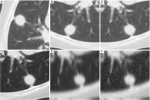
Data augmentation for training the deep learning models was carried out on the train set in five sequential steps: (I) random rotation by 90°, 180° or 270°; (II) random vertical or horizontal flip; (III) random gamma correction with γ ∈ [0.5, 1.5]; (IV) random Gaussian smoothing with σ ∈ [0.5, 2.0] and (V) addition of random Gaussian noise with σ=0.025 and amplitude of the error rescaled to 255. The effects on a sample image are shown in Figure 2A,B,C,D,E,F. The steps were carried out in the above sequence and in a recursive manner—i.e., the output of one step was the input to the following one, the input to the first step being the original images of the train or validation group. At each step half of the images was randomly picked for augmentation while the remaining half passed on to the following step unchanged. The final number of images in the augmented train set was 1,127.

Figure 2 Effects of data augmentation on a sample image. The transformation were applied in a recursive manner—i.e., the output of each step was the input to the following one. In column-wise order: (A) original image; (B) image after anti-clockwise rotation by 90°; (C) after left-right flip; (D) after gamma correction (γ=1.5); (E) after Gaussian smoothing (σ=2.0) and (F) after the addition of Gaussian random noise (µ=0, σ=0.025).

Independent evaluation dataset

An independent evaluation dataset based on the LIDC-IDRI repository (50,51) was also considered in the present study. This included 259 planar axial patches again of dimension 64 px × 64 px from 100 CT scans representing solid and sub-solid nodules (texture index ≥4). For compatibility with the in-house dataset described above, only scans with slice thickness between 3.0 and 4.0­ mm were considered; furthermore, the windowing and resampling settings used to convert the original dicom data from Hounsfield Units to grey-scale values also remained unchanged.

The reference segmentation of each nodule (ground-truth) was obtained by blending the annotations available within the LIDC-IDRI dataset at a consensus level of 0.5. Therefore, a voxel was considered ‘lesion’ if it was marked as such in at least half of the annotations available for the corresponding nodule, ‘not-lesion’ otherwise.

Data availability

For reproducible research purposes, all the images and segmentation masks (ground truth) of the proprietary and independent dataset are available as supplementary material (respectively ‘LNSEG-SSR-1.zip’ and ‘LNSEG-LIDC-IDRI-SSR-1.zip’).

Segmentation procedure

The proposed semi-automatic (‘one-click’) procedure only requires the user to select a point around the centre of the region of interest (Figure 3). It works as follows: (I) on the region of interest (Figure 3A) the user selects a seed point around the centre of the nodule (Figure 3B); (II) the segmentation algorithm partitions the input image into a number of connected regions (blobs—Figure 3C) and (III) only the blob containing the seed pixel is retained whereas the others are discarded (Figure 3D). Depending on the specific algorithm used (step 2) the seed point can also be an input the segmentation algorithm.

Figure 3 Summary scheme of the semi-automated (‘one-click’) segmentation procedure: (A) original image; (B) original image with the seed pixel selected by the user; (C) blobs produced by the segmentation algorithm and (D) final result.

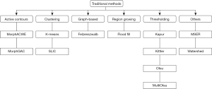
Conventional approaches

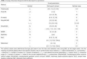
We considered 12 classic image segmentation approaches as detailed below (see Figure 4 for a taxonomy). For the methods that depend on parameters (Table 1) the optimal values were determined via grid search over the train and validation images using Sørensen-Dice coefficient (DSC) as the target measure (more on this in “Experiments”).

Figure 4 Taxonomy of the hand-designed methods. MorphACWE, morphological active contours without edges; MorphGAC, morphological geodesic active contours; MSER, maximally stable extremal regions; SLIC, simple linear iterative clustering.

Table 1 Tuning of the hand-designed methods that depend on parameters
Full table

Active contours

The basic idea behind active contour models (or snakes) is deforming an initial curve towards the boundary of the region/object to be detected. The starting curve can be either internal or external to the region of interest; as a result the contour will either expand or shrink toward the boundary of the object. The evolution of the curve is governed by some functional F, defined in a way such as that the minimum of F falls on the boundary of the region of interest. In their original formulation active contours required solving a system of partial differential equations (PDE), which is computationally expensive and prone to numerical instability. Later on it was shown that solving the PDE could be avoided by using morphological operators (45). These proved infinitesimally equivalent to the PDE but computationally cheaper and free from instability problems. Here we considered two morphology-based implementation of active contours; in both cases the initial curve was a circle of radius r=3 px centred on the pixel selected by the user (see Figure 3B).

Morphological active contours without edges (MorphACWE)

This model, originally proposed by Chan and Vese (52), is based on the assumption that the image to segment is formed by two regions of approximately uniform intra-region intensities different from one another. Say the contour splits the image into and inside and outside region, and let these be Ci and Co respectively. Let also F(Ci), F(Co) indicate the sum of the within-region absolute difference between the intensity of each pixel and the average intensity over that region. The functional is defined as F = λ₁F(Ci) + λ₂F(Co), were λ₁, λ₂ are two positive parameters to be determined. In (52) the authors recommended λ₁=λ₂=1.0; in our experiments we sought the best combination through grid search over λ₁, λ₂ ∈ {1.0, 2.0, 4.0}, which returned λ₁=1.0, λ₂=4.0 as the optimal values. Another parameter to set is the number of iterations to run (N_i), for which we found the optimal value N_i=10 again through grid search over N_i ∈ {10, 20, 40}.

Morphological geodesic active contours (MorphGAC)

In GAC the minimisation of F leads to determining a geodesic curve in a Riemannian space in which the metric is induced by some image features, like the edges (53,54). The parameters to tune, in this case, are the number of iterations to run (N_i, same as in MorphACWE) and the balloon force (f_b). The latter guides the contour in the regions of the image where the gradient is too small (negative values will shrink the contour, positive values will expand it). The optimal value f_b=0.5 was determined via grid search over f_b ∈ {–1.0, –0.5, 0.0, 0.5, 1.0}. As for MorphACWE we found the optimal number of iterations N_i=10 via grid search over Ni ∈ {10, 20, 40}.

Clustering

K-means

This is a classic approach to clustering—i.e., given an arbitrary number of observations and k classes choose k points (cluster centroids) such as that the sum of the distance between each point and the closest centroid is minimal (55). In image segmentation the point coordinates are usually the colour triplets or the intensity values in the case of grey-scale images. In the original formulation the algorithms starts by randomly choosing k initial centroids and by assigning each point to the closest centroid. Then at each step the centroids are recomputed as the centres of mass of the points assigned to each of them. The process exits when there is no point reassignment at some step, or if the maximum allowed number of iterations is reached. The main input parameter to the algorithm is the number of classes, which we determined through grid search over k ∈ {4, 8, 12, 16}. This returned k=8 as the optimal value. For cluster initialisation we used ‘k-means++’ selection (56) which improves convergence.

Simple linear iterative clustering (SLIC)

This iterative clustering algorithm (57) is an evolution of the K-means with two major differences: (I) it employs a weighted distance that combines colour (luminance in this case) and spatial proximity; (II) searches a limited region around the nearest cluster, whereas K-means searches the entire image. The balance between intensity and space proximity is regulated by a compactness parameter c, with higher values giving more weight to space proximity. The algorithm starts by sampling k initial cluster centroids on a regular grid across the input image, then at each step associates each pixel to the nearest centre within the search region. There are two input parameters to SLIC: the number of clusters (also referred to as ‘superpixels’) and the compactness—respectively k and m in the notation used in (57). The best combination was determined via grid search over k ∈ {4, 8, 12, 16} and c ∈ {0.1, 1, 10, 100}, which returned k=16 and c=1.0.

Graph-based

Felsenszwalb’s graph-based image segmentation

Consider G = (V, E) an undirected graph where the vertices vi ∈ V represent the elements (pixels) to be segmented and the edges eij = (vi, vj) the connections between pairs of elements. Let also wij be the weight associated with each such connections, which, for greyscale images is the absolute difference between the intensity level of the connected pixels. Define a segmentation S as a partition of V into components Ck ∈ S such that each Ck is a connected component in a sub-graph of G. Say a segmentation S is too fine when there is some pairs of regions Ca, Cb for which there is no evidence of a boundary between them, and too coarse if there exists a refinement of S that is not too fine. A segmentation produced by Felzenszwalb’s method obeys the properties of being not too coarse or too fine (58). The main parameter governing the algorithm is the scale of observation s, with higher values resulting in fewer and larger segments. Here we determined the optimal value s=2.0 through grid-search over s ∈ {0.5, 1.0, 2.0, 4.0}. We also set a minimum area threshold Am =25 px as a cut-off value for the resulting segments, and σ=1 as the standard deviation of the Gaussian kernel used in preprocessing.

Region growing

Flood fill

Flood fill generates blobs by merging adjacent pixels based on their similarity to an initial seed. Conceptually, this is very similar to the ‘paint bucket’ tool available in many graphic editors. The input parameters are: the seed pixel (which is selected manually by the operator—see Figure 3B), the connectivity (d) and the tolerance (τ). The connectivity determines the neighbourhood of each pixel, and, consequently the possible path(s) that link the target pixels to the seed: adjacent pixels whose mutual distance is less than or equal to d are considered neighbours. The tolerance establishes the range within which the target pixels and the seed are considered equal: pixels connected to the seed and with values within ±τ from that of the seed are merged. In the experiments we determined the optimal values d=1 and τ=16 through grid search respectively over d ∈ {1, 2} and τ ∈ {2, 4, 8, 16}.

Thresholding

Thresholding consists of partitioning the input image by applying one or more cut-off values (thresholds) on the grey-level intensities. Given a set of thresholds ti: {0 ≤ t1, …, tN ≤ 2n–1} the 0-, N- and i-th class respectively will be the sets of pixels having grey-level intensities below t1, above or equal to tN and in the [ti, ti+1] interval, where n indicates the bit depth of the input image. The case N=1 is usually referred to as single-level thresholding, the case N>1 as multi-level thresholding. Here we considered three classic single-level thresholding methods (Otsu’s, Kapur’s and Kittler’s) and the multi-level version of Otsu’s.

Otsu

Otsu’s is possibly one of the most used approaches to image thresholding. The method seeks the value that minimizes the weighted sum of the between-class variance in the background and foreground pixels (59). It gives satisfactory results when the intensity distribution approaches a bimodal and the relative proportion of foreground and background is approximately the same for the two classes (60).

Kapur

This method, also referred to as entropic thresholding (60,61), considers the grey-level histograms of the foreground and background classes as signals, and seeks the value that maximises the sum of the entropy of the two signals (62).

Multi-Otsu

This is an extension of Otsu’s approach for N>1: in this case the algorithm seeks the set of threshold values that minimise the weighted sum of the parwise between-class variance (63). The optimal number of classes N=4 was determined via grid search over N ∈ {3, 4}.

Maximally stable extremal regions (MSER)

MSER are a method for blob detection originally introduced by Matas et al. (64). The basic idea behind MSER is the following. Imagine we binarize a greyscale image with a variable threshold; as the threshold varies within a given range (let ∆ be the range) there will be some connected components of the binarized image that will remain approximately the same: these are stable regions. Among them, maximally stable regions are those exhibiting the lowest area variation when the threshold varies. A stable region is also extremal if the intensity of all its pixels is either higher (bright extremal regions) or lower (dark extremal regions) than that of the surrounding pixels.

In the experiments the value of ∆ was determined through grid search over ∆ ∈ {2, 4, 6, 8}, which returned ∆=2 as the optimal value. The other parameters were: minimum (maximum) area cut-off value for the detected blobs =10 px (25% of the area of the input image), maximum variation (absolute stability score) of the regions =0.25 and minimum diversity =0.2 (when the relative area difference between two nested regions was below this threshold only the most stable one was retained).

Watershed

In watershed segmentation the input image is regarded as an elevation map, that is to say the equivalent of a topographic landscape with ridges and valleys. The objective of the algorithm is to decompose the image into catchment basins and watersheds (65,66). Formally, for a local minimum m, a catchment basin is defined as the set of pixels which are topographically closer to m—i.e., those pixels having the path of steepest descent terminates at m. The procedure requires an external input from the user who needs to select a marker within the region of interest (see Figure 3). Although the method can be applied to the original greyscale image with no pre-processing, it usually works better if a gradient operator is applied first. This proved true for the application studied here, therefore we preliminary computed the local gradient using a circular neighbourhood of radius r=2 px. The value was determined through grid search over r ∈ {2, 3, 4}. As in SLIC, the segmentation results can be further improved by introducing a compactness parameter c: in this case the tuning returned c=0.1 as the optimal value after grid search over c ∈ {0.1, 1.0, 10.0, 100.0}.

Deep learning methods

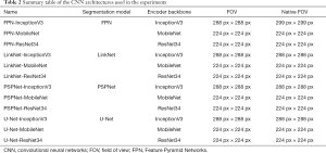
We assembled 12 CNN by combining four standard segmentation models and three well-known backbone encoders as detailed in the following subsections (see also Table 2 for a round-up). By design we kept the input size (receptive field) of each network as close as possible to that of the corresponding backbone encoder while complying with the constraints given by the segmentation models used. [Specifically, Feature Pyramid Networks (FPN), LinkNet and U-Net require the height and width of the input images to be multiple of 32; PSPNet to be multiple of 48]. Albeit this restriction is not strictly necessary, we made this choice because the backbone encoders come with pre-trained weights optimised for their native resolutions. Consequently, we rescaled the input (greyscale) and output (segmented) images accordingly. Also, since all the backbone architecture used are designed for three-channel images, we preliminary converted the input grey-scale images by repeating the two-dimensional array along the third dimension. Finally, we considered nodule segmentation as a one-class classification problem, therefore defined the output of each network as a single-channel layer with sigmoid activation. The final labels were generated by rounding the output to the nearest integer (0= not nodule, 1= nodule).

Table 2 Summary table of the CNN architectures used in the experiments
Full table

Segmentation models

CNN for image segmentation typically rely on an encoder-decoder architecture (59). The encoder (down-sampling or contracting path) gradually reduces the size of the representation while capturing semantic/contextual information; the decoder (up-sampling or expanding path) projects back the representation to its original size, this way producing pixel-wise predictions. The basic building blocks of CNN for image segmentation are convolutional, pooling and transposed (backwards) convolutional layers. Other elements like skip connections enable direct links between the down-sampling and up-sampling path (62,67). A number of variations on this idea have been proposed in the literature, and in this work we considered four different architectures: U-Net, LinkNet, FPN and Pyramid Scene Parsing Network (PSPNet). Below we summarise the basics of each architecture and refer the reader to the given references for further details and technicalities.

U-Net and LinkNet have a very similar structure—that of a ‘ladder’ network (68). In this architecture the encoder and decoder ideally represent the rails of the ladder and the rungs their connections. The U-Net has symmetric contracting and expanding paths, and concatenates the feature maps from the encoder to the corresponding up-sampled maps from the decoder by copy and crop (69,70). This allows the decoder to reconstruct relevant features that are lost when pooled in the encoder. The LinkNet (71) has a very similar layout and differs from the U-Net only for a number of minor changes in the encoder and decoder structure.

Differently from U-Net and LinkNet, FPN and PSPNet are based on combining information at different resolutions via pyramidal decomposition. This concept, which was for long a mainstay of image analysis during the hand-designed era (72,73), translates seamlessly to deep learning due to the intrinsically multi-resolution nature of convolutional networks. FPN were originally designed for multi-scale object detection (74), an objective they achieve by computing feature maps of different size with a scaling ratio of two. This architecture was later on adapted to semantic segmentation by resizing each-single scale prediction to the field-of-view of the network and summing up the results [panoptic configuration (75)]. Pyramid Parsing Networks (76) work on a similar idea, but in this case they obtain the pyramidal decompositions by pooling the feature map produced by the encoder at different sizes. They then feed the results to a convolution layer which up-samples the results to make them the same size as receptive field of the network.

Encoder backbones

For the encoder backbones we employed the fully-convolutional version of three well-established architectures: ResNet34, InceptionV3 and MobileNet. These models have been described at length in a number of papers (36,77-79) therefore we shall not go into further details here. Let us just recall that the residual networks (ResNets) were specifically designed for accuracy, the MobileNets for computational efficiency, and the Inception for a balance between the two. For all the models the starting values of the weights were those resulting from training the original CNN on the ImageNet dataset [ILSVRC 2020 (80)]. Further details about the implementation are given in the Experiments.

Training

We evaluated two different training strategies: (I) full training, in which all the trainable parameters of the networks were liable to be modified during the training phase; and (II) fine tuning, where only the decoder parameters could be modified. In both cases the starting values for the encoder weights were the pre-defined ones obtained by training on the ImageNet dataset. We used Adam optimisation with an initial learning rate of 0.001 and exponential decay rate for the first and second moment estimates respectively of 0.9 and 0.999. The target function for the optimisation process was Dice loss (definition to follow). We processed the train and validation images by batches of two, allowed a maximum of 50 epochs and triggered early stopping if the validation loss did not improve by more than 0.5% for more than five consecutive epochs.

Experiments

Evaluation metrics

Following the same approach adopted in related works (33,41,44) we used Sørensen-Dice coefficient (DSC in the remainder) as the primary metric for evaluating the overlap between the manually segmented regions (ground truth) and the automatically segmented ones. For any two finite sets A, B DSC is defined as follows (81):

DSC(A,B)=2|A∩B||A|+|B|[1]

where |X| indicates the cardinality of X. Let us recall that DSC has values in [0, 1], and that 1 indicates perfect overlap between A and B; 0 no overlap. The Dice loss is (1 – DSC).

Statistical analysis

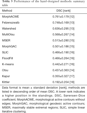
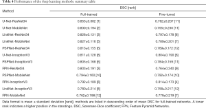
All the methods were pairwise evaluated through non-parametric Wilcoxon-Mann-Withney test at a significance level α=0.05 by comparing the DSC achieved by the two methods on each image tested. For each comparison a +1 was assigned to the best method if one of the two was significantly better than the other, nil to the other. In case of a tie (no statistically significant difference between the two methods) both received nil. An overall ranking was finally determined by summing up the points received by each method and sorting accordingly (see Tables 3,4).

Table 3 Performance of the hand-designed methods: summary table
Full table

Table 4 Performance of the deep learning methods: summary table
Full table

Implementation and execution

We carried out the experiments on a laptop PC equipped with Intel^® Core^TM i7-9750H CPU @ 2.60 GHz, 32 GB RAM, NVIDIA Quadro T1000 (4 GB) graphic card and Windows 10 Pro 64-bit operating system. For the coding we used Python 3.8.6 with functions from scikit-image 0.17.2 (82) and scikit-learn 0.23.3 (83) for the implementation of the hand-designed methods, and from the Segmentation Models package (84) for the deep networks. The training of all the CNN took approximately 15 hrs using GPU acceleration; parameter optimisation for the conventional methods less than 1 h.

Results

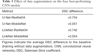
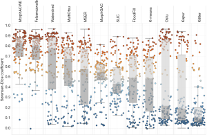
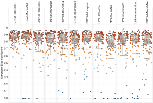
Tables 3-5 and Figures 5,6 summarise the results of the experiments. As can be seen, there is little doubt that the methods based on deep learning outperformed the conventional ones. Notably, even the worst-performing full-trained network (FPN-MobileNet, Table 4) attained better average DSC than the best-performing engineered approach (MorphACWE, Table 3). The box-plots in Figures 5,6 also indicate that the deep learning methods had much narrower dispersion than the engineered ones. As for the convolutional networks, the combinations U-Net/LinkNet segmentation models with ResNet34/MobileNet encoder backbones provided the best results. It is also evident from Table 4 that training the whole networks (full-training) was preferable to training the decoder only (fine-tuning). We also explored the effects of data augmentation and observed that this improved the overall outcome—as one would expect (Table 5). Notably, the difference was higher for the ResNet34 backbone encoder than the MobileNet, a result consistent with the higher complexity of the former.

Table 5 Effect of data augmentation on the four best-performing CNN models
Full table

Figure 5 Performance of the conventional methods: box plots. Each dot represents one image of the test set. Methods are listed in descending order of mean DSC from left to right. DSC, Sørensen-Dice coefficient.

Figure 6 Performance of the methods based on deep learning: box plots. Each dot represents one image of the test set. Methods are listed in descending order of mean DSC from left to right. DSC, Sørensen-Dice coefficient.

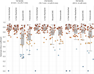
To assess any potential correlation between segmentation accuracy and nodule size we split the test set into three size groups based on the axial diameter of the nodules: axial diameter between 5.0 and 16.1 mm (1st tercile), between 16.1 and 22.5 mm (2nd tercile) and between 22.5 and 40 mm (3rd tercile). Then we tested the four best-performing approaches (two conventional and two based on deep learning) on the three groups. The results (Figure 7) indicate that the methods based on deep learning were generally superior to the conventional ones in all the three groups.

Figure 7 Performance of the two best-performing conventional and deep learning methods broken down by nodule size. From left to right: small nodules (1st tercile), medium-size nodules (2nd tercile) and large nodules (3rd tercile). Symbol d indicates the axial diameter of the nodule.

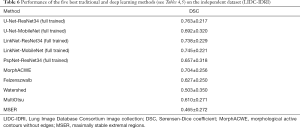
The overall performance of the 10 best-performing methods (five conventional and five based on deep learning) was also evaluated on the external test set based on the LIDC-IDRI repository (“Methods” section). We can see from Table 6 that the results obtained on this dataset confirm the overall trend—i.e., that convolutional networks achieved higher performance. Among the hand-designed methods it is to note the good results achieved by MorphACWE.

Table 6 Performance of the five best traditional and deep learning methods (see Tables 4,5) on the independent dataset (LIDC-IDRI)
Full table

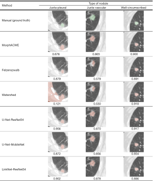
Figure 8 shows the ground truth (manual segmentation) along with the segmentation results obtained with the three best performing engineered methods (MorphACWE, Felzenszwalb and Watershed) and the three best deep networks (U-Net-ResNet34, U-Net-MobileNet and LinkNet-ResNet34) respectively on one juxta-pleural, one juxta-vascular and one well-circumscribed nodule.

Figure 8 Qualitative analysis of the segmentation results obtained with the three best-performing conventional and deep learning methods (Tables 3,4) on juxta-pleural, juxta-vascular and well-circumscribed nodules. The green overlays indicate manual segmentation (ground truth), the orange ones the result of each method. The corresponding DSC is reported beneath each picture. DSC, Sørensen-Dice coefficient.

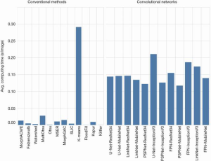
As for the computational demand (Figure 9), we found that the convolutional networks were significantly slower than the conventional methods, as one would reasonably expect. Furthermore, training the networks was significantly more demanding than finding the best parameter combinations for the conventional methods.

Figure 9 Computational demand (average processing time per image) by method. The chart does not include the computing time needed for training the convolutional networks and for optimising the parameters of the traditional methods (see “Implementation and execution” section for details on this).

Albeit the figures are not directly comparable due to differences in the experimental settings and data, it is nonetheless useful to analyse our results in the context of the recent literature. We see that Rocha et al. (39) achieved 0.830 DSC with a custom U-Net architecture (which is close to the best result obtained here), Huang et al. (41) 0.793 with a customised fully-convolutional network based on VGG16 (85) as encoder backbone, and Wang et al. (43) 0.822 again with a bespoke convolutional network. As for hand-designed methods, Mukhopaday (86) recorded average 0.610 DSC through a multi-step hand-designed approach, Rocha et al. (39) 0.663 with sliding band filter, Lassen et al. (87) 0.684 again with a tailored multi-step procedure, and Kim et al. (44) 0.808 by level-set active contours (note that the latter two were obtained respectively on sub-solid and ground-glass nodules).

Discussion

During the last few years research in the field has been gradually shifting its focus from conventional approaches to deep learning methods. The classic methods employ hand-designed data transformations (feature engineering) which are based on some domain-specific knowledge. These methods tend to be computationally cheap and require little or no training. Deep learning, on the other hand, can automatise the feature engineering process—provided that enough data are available. This goal is achieved through the combination of standard basic modules (layers) which contain a number of parameters whose values need to be determined via training. One major advantage of this procedure is that it simplifies the processing pipeline by replacing it with a standard, end-to-end learning model. The question investigated in this paper was the following: is it possible to put together convolutional networks in a relatively simple way, train them on reasonably small amount of data and obtain segmentation accuracy comparable or better than provided by conventional methods? Our results suggest a positive answer, and also indicated a resounding superiority of the deep learning approaches. We think this outcome is remarkable, particularly if we consider that the convolutional networks used here were based on combinations of standard segmentation models and backbone encoders, and that we trained the nets on a relatively small amount of data. This also casts doubts whether designing task-specific convolutional models is strictly necessary, provided that the combination of existing architectures trained on domain-specific data seems to give satisfactory results.

Segmentation of lung nodules is a crucial step in the radiomics pipeline and plays an important role in the management of patients with suspect LC. Unfortunately, the process is tedious and time-consuming when performed manually, puts a lot of pressure on the personnel and suffers from a number of drawbacks such as subjective evaluation and lack of repeatability. Furthermore, the task is complicated by the great variability of the shape, size, texture and location of the nodules. In this paper we have presented a pipeline for semi-automated segmentation of pulmonary nodules which requires very little intervention from the user. The proposed solution can be wired with conventional, hand-designed image descriptors as well as deep learning methods. The main objective of this work was to comparatively evaluate the effectiveness of these two classes. To this end we considered 12 conventional segmentation methods and as many deep learning architectures. The main outcome was the clear superiority of the deep learning methods over the hand-designed ones. Although this was not unexpected—actually the recent literature already points in that direction (39,41,43)—it was certainly remarkable that state-of-the-art performance could be achieved via standard deep learning architectures and by training them on a relatively small amount of data.

Although the results found here are interesting and promising, the present work is not exempt from limitations. Among them are the relatively small sample size and the fact that our datasets was mostly composed of solid nodules. The results should therefore validated in future larger studies featuring also sub-solid and ground-glass nodules. Although the superiority of deep learning was clear in this work, it seems reasonable to speculate that at least some of the knowledge developed during the hand-crafted era could be conveniently carried over to the new age. One interesting direction for future studies could therefore be the integration of deep learning with conventional methods for the segmentation of lung nodules. The discussion on the segmentation accuracy as a function of nodule location was based on visual (qualitative) evaluation of the results: a quantitative analysis could be another interesting subject for future studies.

Acknowledgments

Figures 5-7,9 were generated using Tableau Desktop, Professional Edition. The authors wish to thank Tableau Software LLC, CA, USA, for providing a free license of the tool for research purposes.

Funding: This work was partially supported by the Università degli Studi di Sassari, Italy, within the framework ‘Fondo di Ateneo per la Ricerca 2020’ and by the Department of Engineering, Università degli Studi di Perugia, Italy, through the project ‘Shape, colour and texture features for the analysis of two- and three-dimensional images: methods and applications’ (Fundamental Research Grants Scheme 2019).

Footnote

Conflicts of Interest: All authors have completed the ICMJE uniform disclosure form (available at http://dx.doi.org/10.21037/qims-20-1356). The authors have no conflicts of interest to declare.

Ethical Statement: The study was conducted in accordance with the Declaration of Helsinki (as revised in 2013) and its later amendments or ethical standards. Ethical approval was not required as this was a retrospective study involving data analysis in anonymous form. For the same reasons, the requirement to obtain informed consent was waived. All patient data were treated following the local privacy regulations.

Open Access Statement: This is an Open Access article distributed in accordance with the Creative Commons Attribution-NonCommercial-NoDerivs 4.0 International License (CC BY-NC-ND 4.0), which permits the non-commercial replication and distribution of the article with the strict proviso that no changes or edits are made and the original work is properly cited (including links to both the formal publication through the relevant DOI and the license). See: https://creativecommons.org/licenses/by-nc-nd/4.0/.

References

1. American Cancer Society. Key Statistics for Lung Cancer. 2020. Available online: https://www.cancer.org/cancer/lung-cancer/about/key-statistics.html (Last visited on 25 Nov. 2020).
2. American Lung Association. Lung cancer fact sheet. 2020. Available online: https://www.lung.org/lung-health-diseases/lung-disease-lookup/lung-cancer/resource-library/lung-cancer-fact-sheet (Last visited on 16 Nov. 2020).
3. American Cancer Society. Lung Cancer Survival Rates. 2019. Available online: https://www. cancer.org/cancer/lung-cancer/detection-diagnosis-staging/survival-rates.html (Last visited on 25 Oct. 2019).
4. Walter JE, Heuvelmans MA, Oudkerk M. Small pulmonary nodules in baseline and incidence screening rounds of low-dose CT lung cancer screening. Transl Lung Cancer Res 2017;6:42-51. [Crossref] [PubMed]
5. Bueno J, Landeras L, Chung JH. Updated Fleischner society guidelines for managing incidental pulmonary nodules: common questions and challenging scenarios. Radiographics 2018;38:1337-50. [Crossref] [PubMed]
6. Avanzo M, Stancanello J, Pirrone G, Sartor G. Radiomics and deep learning in lung cancer. Strahlentherapie und Onkologie 2020;196:879-87. [Crossref] [PubMed]
7. Hassani C, Varghese BA, Nieva J, Duddalwar V. Radiomics in pulmonary lesion imaging. AJR Am J Roentgenol 2019;212:497-504. [Crossref] [PubMed]
8. Bianconi F, Palumbo I, Fravolini ML, Chiari R, Minestrini M, Brunese L, Palumbo B. Texture analysis on [18F]FDG PET/CT in non-small-cell lung cancer: correlations between PET features, CT features, and histological types. Mol Imaging Biol 2019;21:1200-9. [Crossref] [PubMed]
9. Bianconi F, Fravolini ML, Bello-Cerezo R, Minestrini M, Scialpi M, Palumbo B. Evaluation of shape and textural features from CT as prognostic biomarkers in non-small cell lung cancer. Anticancer Res 2018;38:2155-60. [PubMed]
10. Scrivener M, de Jong EEC, van Timmeren T. Pieters, Ghaye B, Geets X. Radiomics applied to lung cancer: a review. Transl Cancer Res 2016;5:398-409. [Crossref]
11. Bashir U, Siddique MM, McLean E, Goh V, Cook GJ. Imaging heterogeneity in lung cancer: Techniques, applications, and challenges. AJR Am J Roentgenol 2016;207:534-43. [Crossref] [PubMed]
12. Palumbo B, Bianconi F, Palumbo I, Fravolini ML, Minestrini M, Nuvoli S, Stazza ML, Rondini M, Spanu A. Value of shape and texture features from 18F-FDG PET/CT to discriminate between benign and malignant solitary pulmonary nodules: an experimental evaluation. Diagnostics (Basel) 2020;10:696. [Crossref] [PubMed]
13. Balagurunathan Y, Schabath MB, Wang H, Liu Y, Gillies RJ. Quantitative imaging features improve discrimination of malignancy in pulmonary nodules. Sci Rep 2019;9:8528. [Crossref] [PubMed]
14. Wu W, Pierce LA, Zhang Y, Pipavath SNJ, Randolph TW, Lastwika KJ, Lampe PD, Houghton AM, Liu H, Xia L, Kinahan PE. Comparison of prediction models with radiological semantic features and radiomics in lung cancer diagnosis of the pulmonary nodules: a case-control study. Eur Radiol 2019;29:6100-8. [Crossref] [PubMed]
15. Chen CH, Chang CK, Tu CY, Liao WC, Wu BR, Chou KT, Chiou YR, Yang SN, Zhang G, Huang TC. Radiomic features analysis in computed tomography images of lung nodule classification. PLoS One 2018;13:e0192002 [Crossref] [PubMed]
16. Dennie C, Thornhill R, Sethi-Virmani V, Souza CA, Bayanati H, Gupta A, Maziak D. Role of quantitative computed tomography texture analysis in the differentiation of primary lung cancer and granulomatous nodules. Quant Imaging Med Surg 2016;6:6-15. [PubMed]
17. Hawkins S, Wang H, Liu Y, Garcia A, Stringfield O, Krewer H, Li Q, Cherezov D, Gatenby RA, Balagurunathan Y, Goldgof D, Schabath MB, Hall L, Gillies RJ. Predicting malignant nodules from screening CT scans. J Thorac Oncol 2016;11:2120-8. [Crossref] [PubMed]
18. Han F, Wang H, Zhang G, Han H, Song B, Li L, Moore W, Lu H, Zhao H, Liang Z. Texture feature analysis for computer-aided diagnosis on pulmonary nodules. J Digit Imaging 2015;28:99-115. [Crossref] [PubMed]
19. Bianconi F, Palumbo I, Spanu A, Nuvoli S, Fravolini ML, Palumbo B. PET/CT radiomics in lung cancer: an overview. Appl Sci 2020;5:1718. [Crossref]
20. Bianconi F, Fravolini ML, Palumbo I, Palumbo B. Shape and texture analysis of radiomic data for computer-assisted diagnosis and prognostication: an overview. In: Rizzi C, Andrisano AO, Leali F, Gherardini F, Pini F, Vergnano A, editors. Proceedings of the International Conference on Design Tools and Methods in Industrial Engineering (ADM). Lecture Notes in Mechanical Engineering. Moden: Springer, 2019:3-14.
21. Huang Q, Lu L, Dercle L, Lichtenstein P, Li Y, Yin Q, Zong M, Schwartz L, Zhao B. Interobserver variability in tumor contouring affects the use of radiomics to predict mutational status. J Med Imaging (Bellingham) 2018;5:011005 [PubMed]
22. van Velden FHP, Kramer GM, Frings V, Nissen IA, Mulder ER, de Langen AJ, Hoekstra OS, Smit EF, Boellaard R. Repeatability of radiomic features in non-small-cell lung cancer [18F]FDG-PET/CT studies: impact of reconstruction and delineation. Mol Imaging Biol 2016;18:788-95. [Crossref] [PubMed]
23. Lee SLA, Kouzani AZ, Hu EJ. Automated detection of lung nodules in computed tomography images: a review. Mach Vis Appl 2012;23:151-63. [Crossref]
24. Zheng L, Lei Y. A review of image segmentation methods for lung nodule detection based on computed tomography images. Shanghai: Proceedings of the 2nd International Conference on Electronic Information Technology and Computer Engineering, 2018;232:02001.
25. Sivakumar S, Chandrasekar C. Lung nodule segmentation through unsupervised clustering models. Tamil Nadu: Proceedings of the International Conference on Modelling Optimization and Computing, 2012;38:3064-73.
26. Tsou CH, Lor KL, Chang YC, Chen CM. Region-based graph cut using hierarchical structure with application to ground-glass opacity pulmonary nodules segmentation. Lake Buena Vista: Proceedings of Medical Imaging 2013: Image Processing. Image Processing 2013;8669:866906
27. Lee CH, Jwo JS. Automatic segmentation for pulmonary nodules in CT images based on multifractal analysis. IET Image Process 2020;14:1265-72. [Crossref]
28. Kubota T, Jerebko AK, Dewan M, Salganicoff M, Krishnan A. Segmentation of pulmonary nodules of various densities with morphological approaches and convexity models. Med Image Anal 2011;15:133-54. [Crossref] [PubMed]
29. Han H, Li L, Han F, Zhang H, Moore W, Liang Z. Vector quantization-based automatic detection of pulmonary nodules in thoracic CT images. Seoul: Proceedings of the 60th IEEE Nuclear Science Symposium and Medical Imaging Conference, 2013:6829365.
30. Ren H, Zhou L, Liu G, Peng X, Shi W, Xu H, Shan F, Liu L. An unsupervised semi-automated pulmonary nodule segmentation method based on enhanced region growing. Quant Imaging Med Surg 2020;10:233-42. [Crossref] [PubMed]
31. Aresta G, Cunha A, Campilho A. Detection of juxta-pleural lung nodules in computed tomography images. Orlando: Proceedings of Medical Imaging 2017 Computer-Aided Diagnosis 2017;10134:101343N
32. Nithila EE, Kumar SS. Segmentation of lung nodule in CT data using active contour model and Fuzzy C-mean clustering. Alex Eng J 2016;55:2583-8. [Crossref]
33. Kalpathy-Cramer J, Zhao B, Goldgof D, Gu Y, Wang X, Yang H, Tan Y, Gillies R, Napel S. A comparison of lung nodule segmentation algorithms: methods and results from a multiinstitutional study. J Digit Imaging 2016;29:476-87. [Crossref] [PubMed]
34. Alilou M, Kovalev V, Snezhko E, Taimouri V. A comprehensive framework for automatic detection of pulmonary nodules in lung CT images. Image Anal Stereol 2014;33:13-27. [Crossref]
35. LeCun Y, Bengio Y, Hinton G. Deep learning. Nature 2015;521:436-44. [Crossref] [PubMed]
36. Alom MZ, Taha TM, Yakopcic C, Westberg S, Sidike P, Nasrin MS, Hasan M, Van Essen BC, Awwal AAS, Asari VK. A state-of-the-art survey on Deep Learning theory and architectures. Electronics 2019;8:292. [Crossref]
37. Wu J, Qian T. A survey of pulmonary nodule detection, segmentation and classification in computed tomography with deep learning techniques. J Med Artif Intell 2019;2:20. [Crossref]
38. Pezzano G, Ribas Ripoll V, Radeva P. CoLe-CNN: Context-learning convolutional neural network with adaptive loss function for lung nodule segmentation. Comput Methods Programs Biomed 2021;198:105792 [Crossref] [PubMed]
39. Rocha J, Cunha A, Mendonça AM. Conventional filtering versus U-Net based models for pulmonary nodule segmentation in CT Images. J Med Syst 2020;44:81. [Crossref] [PubMed]
40. Shi Z, Hu Q, Yue Y, Wang Z. AL-Othmani OMS, Li H. Automatic nodule segmentation method for CT images using aggregation-U-Net generative adversarial networks. Sens Imaging 2020;21:39. [Crossref]
41. Huang X, Sun W, Tseng TLB, Li C, Qian W. Fast and fully-automated detection and segmentation of pulmonary nodules in thoracic CT scans using deep convolutional neural networks. Comput Med Imaging Graph 2019;74:25-36. [Crossref] [PubMed]
42. Liu M, Dong J, Dong X, Yu H, Qi L. Segmentation of Lung Nodule in CT Images Based on Mask R-CNN. Fukuoka: Proceedings of the 9th International Conference on Awareness Science and Technology (iCAST), 2018:95-100.
43. Wang S, Zhou M, Liu Z, Liu Z, Gu D, Zang Y, Dong D, Gevaert O, Tian J. Central focused convolutional neural networks: Developing a data-driven model for lung nodule segmentation. Med Image Anal 2017;40:172-83. [Crossref] [PubMed]
44. Kim YJ, Lee SH, Park CM, Kim KG. Evaluation of semi-automatic segmentation methods for persistent ground glass nodules on thin-section CT scans. Healthc Inform Res 2016;22:305-15. [Crossref] [PubMed]
45. Awai K, Murao K, Ozawa A, Komi M, Hayakawa H, Hori S, Nishimura Y. Pulmonary nodules at chest CT: effect of computer-aided diagnosis on radiologists’ detection performance. Radiology 2004;230:347-52. [Crossref] [PubMed]
46. Javaid M, Javid M, Rehman MZ, Shah SI. A novel approach to CAD system for the detection of lung nodules in CT images. Comput Methods Programs Biomed 2016;135:125-39. [Crossref] [PubMed]
47. Kobayashi H, Ohkubo M, Narita A, Marasinghe JC, Murao K, Matsumoto T, Sone S, Wada S. A method for evaluating the performance of computer-aided detection of pulmonary nodules in lung cancer CT screening: detection limit for nodule size and density. Br J Radiol 2017;90:20160313 [Crossref] [PubMed]
48. Wagner AK, Hapich A, Psychogios MN, Teichgräber U, Malich A, Papageorgiou I. Computer-aided detection of pulmonary nodules in computed tomography using ClearReadCT. J Med Syst 2019;43:58. [Crossref] [PubMed]
49. Nioche C, Orlhac F, Boughdad S, Reuze S, Goya-Outi J, Robert C, Pellot-Barakat C, Soussan M, Frouin FE, Buvat I. LIFEx: A freeware for radiomic feature calculation in multimodality imaging to accelerate advances in the characterization of tumor heterogeneity. Cancer Res 2018;78:4786-9. [Crossref] [PubMed]
50. Armato SG III, McLennan G, Bidaut L, McNitt-Gray MF, Meyer CR, Reeves AP, et al. The Lung Image Database Consortium (LIDC) and Image Database Resource Initiative (IDRI): a completed reference database of lung nodules on CT scans. Medical Physics 2011;38:915-31. [Crossref] [PubMed]
51. Clark K, Vendt B, Smith K, Freymann J, Kirby J, Koppel P, Moore S, Phillips S, Maffitt D, Pringle M, Tarbox L, Prior F. The Cancer Imaging Archive (TCIA): maintaining and operating a public information repository. J Digit Imaging 2013;26:1045-57. [Crossref] [PubMed]
52. Chan TF, Vese LA. Active contours without edges. IEEE Trans Image Process 2001;10:266-77. [Crossref] [PubMed]
53. Márquez-Neila P, Baumela L, Alvarez L. A morphological approach to curvature-based evolution of curves and surfaces. IEEE Trans Pattern Anal Mach Intell 2014;36:2-17. [Crossref] [PubMed]
54. Caselles V, Kimmel R, Sapiro G. Geodesic active contours. Int J Comput Vis 1997;22:61-79. [Crossref]
55. Theodoridis S, Koutroumbas K. Pattern recognition. 3rd ed. Cambridge: Academic Press, 2006.
56. Arthur D, Vassilvitskii S. K-means++: The advantages of careful seeding. New Orleans: Proceedings of the Annual ACM-SIAM Symposium on Discrete Algorithms, 2007:1027-35.
57. Achanta R, Shaji A, Smith K, Lucchi A, Fua P, Süsstrunk S. SLIC superpixels compared to state-of-the-art superpixel methods. IEEE Trans Pattern Anal Mach Intell 2012;34:2274-82. [Crossref] [PubMed]
58. Felzenszwalb PF, Huttenlocher DP. Efficient graph-based image segmentation. Int J Comput Vis 2004;59:167-81. [Crossref]
59. Otsu N. Threshold selection method from gray-level histogram. IEEE Trans Syst Man Cybern 1979;SMC-9:62-6. [Crossref]
60. Sezgin M, Sankur B. Survey over image thresholding techniques and quantitative performance evaluation. J Electron Imaging 2004;13:146-68. [Crossref]
61. Kapur JN, Sahoo PK, Wong AKC. A new method for gray-level picture thresholding using the entropy of the histogram. Comput Gr Image Process 1985;29:273-85. [Crossref]
62. Lamba H. Understanding Semantic Segmentation with UNET: A Salt Identification Case Study. Towards Data Science. 2019. Available online: https://towardsdatascience.com/understanding-semantic-segmentation-with-unet-6be4f42d4b47 (Visited on 7 Nov. 2020).
63. Liao PS, Chen TS, Chung PC. A fast algorithm for multilevel thresholding. J Inf Sci Eng 2001;17:713-27.
64. Matas J, Chum O, Urban M, Pajdla T. Robust wide-baseline stereo from maximally stable extremal regions. Image Vis Comput 2004;22:761-7. [Crossref]
65. Roerdink JBTM, Meijster A. The watershed transform: definitions, algorithms and parallelization strategies. Fundam Inform 2000;41:187-228. [Crossref]
66. Preim B, Botha C. Image analysis for medical visualization. In: Preim B, Botha C. editors. Visual computing for medicine: theory, algorithms, and applications. 2nd ed. Waltham: Morgan Kaufman, 2014:111-75.
67. Shelhamer E, Long J, Darrell T. Fully convolutional networks for semantic segmentation. IEEE Trans Pattern Anal Mach Intell 2017;39:640-51. [Crossref] [PubMed]
68. Rasmus A, Valpola H, Honkala M, Berglund M, Raiko T. Semi-supervised learning with Ladder networks. arXiv 2015:1507.02672.
69. Ronneberger O, Fischer P, Brox T. U-net: Convolutional networks for biomedical image segmentation. In: Navab N, Hornegger J, Wells WM, Frangi AF. editors. Medical Image Computing and Computer-Assisted Intervention-MICCAI 2015. Lecture Notes in Computer Science. Cham: Springer, 2015:234-41.
70. Karabaǧ C, Verhoeven J, Miller NR, Reyes-Aldasoro CC. Texture segmentation: An objective comparison between five traditional algorithms and a deep-learning U-net architecture. Appl Sci 2019;9:3900. [Crossref]
71. Chaurasia A, Culurciello E. LinkNet: Exploiting encoder representations for efficient semantic segmentation. St. Petersburg: Proceedings of the IEEE Visual Communications and Image Processing (VCIP), 2017:1-4.
72. Lazebnik S, Schmid C, Ponce J. Beyond bags of features: spatial pyramid matching for recognizing natural scene categories. New York Proceedings of the IEEE Computer Society Conference on Computer Vision and Pattern Recognition 2006;2:2169-78. [Crossref]
73. Adelson EH, Burt PJ, Anderson CH, Ogden JM, Bergen JR. Pyramid methods in image processing. RCA Engineer 1984;29:33-41.
74. Lin TY, Dollár P, Girshick R, He K, Hariharan B, Belongie S. Feature pyramid networks for object detection. Honolulu: Proceedings of the 30th IEEE Conference on Computer Vision and Pattern Recognition, 2017:936-44.
75. Kirillov A, Girshick R, He K, Dollar P. Panoptic feature pyramid networks. Long Beach: Proceedings of the 32nd IEEE/CVF Conference on Computer Vision and Pattern Recognition, 2019:6392-401.
76. Zhao H, Shi J, Qi X, Wang X, Jia J. Pyramid scene parsing network. Honolulu: Proceedings of the 30th IEEE Conference on Computer Vision and Pattern Recognition, 2017:6230-9.
77. Tsang SH. Review: MobileNetV1 – depthwise separable convolution (lightweight model). Towards Data Science. 2018. Available online: https://towardsdatascience.com/review-mobilenetv1-depthwise-separable-convolution-light-weight-model-a382df364b69 (Visited on 9 Nov. 2020).
78. He K, Zhang X, Ren S, Sun J. Deep residual learning for image recognition. In: Las Vegas: Proceedings of the IEEE Computer Society Conference on Computer Vision and Pattern Recognition, 2016:770-8.
79. Szegedy C, Vanhoucke V, Ioffe S, Shlens J, Wojna Z. Rethinking the inception architecture for computer vision. Las Vegas: Proceedings of the IEEE Computer Society Conference on Computer Vision and Pattern Recognition, 2016:2818-26.
80. ImageNet Large Scale Visual Recognition Challenge. 2012. Available online: http://image-net.org/challenges/LSVRC/2012/ (Last visited on 9 Dec. 2020).
81. Verma V, Aggarwal RK. A comparative analysis of similarity measures akin to the Jaccard index in collaborative recommendations: empirical and theoretical perspective. Soc Netw Anal Min 2020;10:43. [Crossref]
82. van der Walt S, Schönberger JL, Nunez-Iglesias J, Boulogne F, Warner JD, Yager N, Gouillart E, Yu T. scikit-image contributors. scikit-image: image processing in Python. PeerJ 2014;2:e453 [Crossref] [PubMed]
83. Pedregosa F, Varoquaux G, Gramfort A, Michel V, Thirion B, Grisel O, Blondel M, Prettenhofer P, Weiss R, Dubourg V, Vanderplas J, Passos A, Cournapeau D, Brucher M, Perrot M, Duchesnay E. scikit-learn: Machine Learning in Python. J Mach Learn Res 2011;12:2825-30.
84. Yakubovskiy P. Python library with Neural Networks for Image Segmentation based on Keras and TensorFlow. Available online: https://github.com/qubvel/segmentation_models (Last visited on 13 Nov. 2020).
85. Chatfield K, Simonyan K, Vedaldi A, Zisserman A. Return of the devil in the details: delving deep into convolutional nets. arXiv 2014:1405.3531.
86. Mukhopadhyay S. A segmentation framework of pulmonary nodules in lung CT images. J Digit Imaging 2016;29:86-103. [Crossref] [PubMed]
87. Lassen BC, Jacobs C, Kuhnigk JM, Van Ginneken B, Van Rikxoort EM. Robust semi-automatic segmentation of pulmonary subsolid nodules in chest computed tomography scans. Phys Med Biol 2015;60:1307-23. [Crossref] [PubMed]