
Automatic segmentation of the left ventricle in echocardiographic images using convolutional neural networks
Introduction
Two-dimensional echocardiography (2D echo) is the most widely used non-invasive method for evaluation of heart disease because of its high temporal resolution [50–250 frames per second (fps)] (1) and short acquisition times (2). 2D echo provides a gray scale image from which anatomical features are identified to assess cardiac functions. Segmentation of the left ventricular (LV) walls in 2D echo is the first step toward quantification of cardiac function, such as ejection fraction (EF) and LV volumes.
At present, semi-automatic or manual delineation conducted by experts are the main boundary identification techniques for 2D echo (3). However, semi-automatic or manual techniques are not only time-consuming but also subjective, which makes them prone to intra- and inter-observer variability (4). Prior to the development of deep learning techniques, methods for automatic LV segmentation could be described as pixel classification (5), image-based methods (6), deformable methods (7), active appearance and shape models (AAM/ASM) (8), and atlas models (9). These methods generated high-quality automatic LV segmentation models on magnetic resonance imaging (MRI) and computerized tomography (CT) images. However, due to speckle noise, brightness inhomogeneities, presence of trabeculae and papillary muscles, and shape and motion variances, these LV segmentation methods suffered from low robustness and accuracy on 2D echo (4). Besides, it was challenging to build a model that would be general enough to cover all possible shapes and dynamics of the LV with previous methods (10). Here, a state-of-the-art deep learning segmentation method is employed for robust and accurate segmentation from 2D echo images.
Medical image analysis has recently been revolutionized through the widespread adoption of deep learning techniques (11). This revolution has primarily been powered by supervised machine learning with convolutional neural networks (CNNs). CNNs typically operate on images and provide one prediction per image sample, e.g., an image class label or quantitation of disease burden (12). Recently, many medical image analyses have employed CNN models (13,14). The most important prerequisite for applying CNNs to the medical image process is to have enough data that are used to train the CNN models. Currently, LV segmentation CNN models are mostly based on MRI or CT images because they are considered as standards (15). The Left Ventricle Segmentation Challenge (LVSC) dataset, organized by the Medical Image Computing and Computer Assisted Intervention Society (MICCAI), consists of 100 fully delineated MRI images of the LV (16). Automated Cardiac Diagnosis Challenge (ACDC) dataset, organized by the MICCAI, consists of 100 patient short-axis MRI images that cover the LV from the base to the apex with a thickness of 5 mm (17). Bai et al. generated a large-scale dataset, which consists of 4,875 patients with 93,500 images, including both short- and long-axis MRI images (18). Zreik et al. made their dataset with cardiac CT angiography (CCTA) short-axis images from 60 patients (19) and trained their CNN model. Lieman-Sifry et al. created a dataset of 1,143 short-axis MRI images (20). With these large datasets, different CNN models are applied to LV segmentation tasks. Çiçek et al. showed that 3D U-net (21) works better than 2D U-net (22) on the ACDC data. Tan et al. used a CNN regression model to segment the LV and parameterize the radius of endocardium and epicardium in short-axis projections with LVSC data (23).
In contrast to MRI, there is no large dataset of 2D echo images. Cardiac Acquisitions for Multi-structure Ultrasound Segmentation (CAMUS) dataset, which consists of 450 patients’ long-axis 2-chamber and 4-chamber projection images, is the only open large dataset (4). For this reason, 2D echo datasets are created for specific studies. Veni et al. constructed 69 2D echo 4-chamber projections for training U-net (24). Zhang et al. used their 2D echo dataset with 214 images of 2-chamber, 141 images of 3-chamber, and 182 images of 4-chamber projections, and 124 short-axis projections, to train their U-net model, and applied the segmented results for auto-diagnosis of the cardiac disease (25). Li et al. used own multi-view dataset, which consists of 9,000 images, and CAMUS dataset for training their multiview recurrent aggregation network (MV-RAN) on the 2-chamber, 3-chamber, and 4-chamber projection images (26,27). However, there was no attempt to segment the standard six 2D echo images, i.e., three short-axis projections and three long-axis projections (28). Furthermore, previous datasets were only concentrated on the end-diastolic and end-systolic images. To segment the LV in this study, U-net (22) and generative adversarial networks model (segAN) (29) were applied on an in-house dataset, which consisted of six standard 2D echo projections, each representing the entire cardiac cycle. Transfer learning was conducted to compensate the limitation of training datasets using CAMUS dataset.
Most of the previous studies for volume analysis using 2D echo images employed single-plane or biplane algorithms. The single-plane area-length algorithm calculated the LV volume by assuming that LV is an ellipsoid and rotating the 4-chamber projection about the long-axis. Biplane Simpson’s algorithm measured the volume of LV by summing volumes of short-axis discs with their radii based on the 4-chamber and 2-chamber long-axis projections. These volumetric studies focused on images at end-systole and end-diastole to calculate the EF. However, visualizing the wall motion and reconstructing the LV geometries over the cardiac cycle is critical for calculating other clinical indices. Also, calculated volumes using these methods showed about 35% error at end-diastole and about 45% error at end-systole compared to the 3D echocardiography or MRI technique (30).
In the current study, six standard projection images, which were segmented by deep learning algorithms (U-net and segAN) over one cardiac cycle, were integrated into a fully automated reconstruction algorithm developed by our group (31). Reconstructed 3D LV geometries over one cardiac cycle facilitated the calculation of clinical indices and tracked the LV wall motion. The results of physiological indices and 3D reconstruction models using automated segmentation versus expert delineation were compared against each other.
Methods
Six standard-projection 2D echo images (three long-axis: 3-, 2- and 4-chamber projections and three short-axis: base, mid, and apex projections) were divided into training and testing datasets. CNN models, which segment the LV were trained on the training dataset. Trained CNN models were evaluated on the test datasets. Segmented images were reconstructed to 3D geometry.
Image acquisition
We obtained the 2D echo scans during ongoing preclinical studies in ten anesthetized open-chest pigs. Porcine models are routinely used in preclinical cardiovascular studies because pig’s cardiovascular anatomy closely replicates human cardiovascular anatomy and physiology (32). However, closed-chest transthoracic ultrasound scans in adult domestic pigs do not reproduce transthoracic echocardiographic scans in humans because of the differences in porcine chest configuration and narrow intercostal spaces (33). Therefore, an open chest setting is often preferred in preclinical studies. Another advantage is that exposing the heart eliminates undesired interposition of lungs, allows unrestricted reproduction of standardized echocardiographic projections, and provides access for experimental instrumentation.
Six standard 2D echo projections of the porcine LV in situ, similar to the ones acquired regularly from human subjects during clinical visits, were captured over one cardiac cycle (R-wave to R-wave) using a Vivid 7 ultrasound system (GE Vingmed Ultrasound AS, Horton, Norway) and an M4S transducer operating at 1.7/3.4 MHz (fundamental/harmonic) frequency. The ultrasound transducer was placed directly on the LV surface to obtain both long- and short-axis images. A transmission gel was applied between the transducer and the LV surface to assure an acoustic coupling. The frame rate was between 36 to 55 fps.
Reference segmentation and contouring protocol
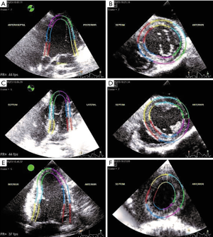
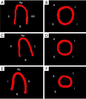
Acquired 2D echo images were delineated by experts using interactive speckle-tracking software (EchoPAC, GE Healthcare). Also the boundary was adjusted, if the tracking was not satisfactory based on a visual inspection by an experienced operator. Manual detection of the myocardium boundary is error-prone and subjective due to typical image dropouts and noise. Therefore, a semi-automatic speckle tracking band was used as a surrogate of the boundary. Speckle tracking methods have been used to obtain LV characteristics in cardiovascular research (34,35). The six standard projections delineated for a given time instant are shown in Figure 1. These delineation images provide the ground truth for the segmentation task.
Deep learning segmentation
Dataset and data augmentation
We employed two different datasets in the current study. First, the CAMUS dataset was used (4). The CAMUS dataset is a fully annotated dataset, which consists of 1,800 long-axis 2-chamber and 4-chamber projections images from 450 patients. The “ground truth image” has four labels, 0: background, 1: LV cavity, 2: LV myocardium, and 3: left atrium. As mentioned above, CAMUS dataset is the only open validated dataset for the 2D echo, but includes only two long-axis projections.
Second, an in-house dataset, which consists of six standard projections, was created and employed. Table 1 shows the total number of images and pigs of the in-house dataset which were used for training and testing of different projections. One porcine data consists of 30 to 40 images over one cardiac cycle with the same time interval. The ground truth images in the in-house dataset have 3 labels: 0: background, 1: LV cavity, and 2: LV myocardium; 75 to 77 images from 2 pigs (different from those used for training) for each projection, i.e., about 20% of total images in the dataset, were assigned to the testing dataset.

Full table
Ronneberger (22) showed that based on the aggressive image augmentation, U-net models could generate promising results with few training images. Several data augmentation techniques were used to overcome the limitations of the training dataset. Rotating, cropping, and blacking-out techniques were used for data augmentation. The training data underwent rotating with 0.7 probability. They were randomly rotated between −25 and 25 degrees. A blank region, created after rotation, was filled using a spline interpolation method. Cropping was conducted with 0.7 probability. It filled out the random amount of missing edges in the images. Finally, a black-out technique by Zhang et al. was applied (25). The technique generated circular areas whose pixel values are zero. In this study, a random diameter circular area was created with random pixel intensities between the maximum and minimum pixel values.
CNN algorithm and training
The previously published U-net (22) and a generative adversarial network (SegAN) (29) models were employed for the LV segmentation. Both models were trained separately for all six standard projections with the in-house training dataset. Transfer learning approach was used for training the models of the long-axis projections. First, the models were trained on the CAMUS dataset (4). Based on these calculated weights, the models were trained with the in-house dataset. Using transfer learning helps to speed up the process of model training and can result in a more accurate segmentation.
To train both CNN models, all input images were resized to 128×128 pixels. Segmented results from both CNN models also had a resolution of 128×128 pixels. The batch size for training both models was 16. The Adam optimizer was used to optimize each model’s loss. Transfer learning was conducted using fine-tuning with reduced learning rate for the long-axis projections. First, our model was trained with 0.001 learning rate on the CAMUS dataset. Next, this trained model was trained with 0.0005 learning rate with our dataset. The training was conducted with Python and TensorFlow. The experiments were performed on NVIDIA TESLA K80 GPU and NVIDIA GeForce GTX 1050 GPU.
Resizing of input images
CAMUS dataset consists of various image sizes, e.g., 486×764. Also, in-house dataset has 648×480. In order to apply these images to CNN models, these images were resized into 128×128 size, which is the same size of both CNN models’ first convolution layer. The original in-house dataset image has 85 pixel/cm pixel spacing. After resizing, input image has 20 pixel/cm pixel spacing. This downsampling may reduce the segmentation performance. This reduction can be solved by increasing the size of the first convolution layer. However, there is a trade off on the memory and computational costs. In this study, we chose 128×128 based on our computational environment.
Original image’s height-width ratio was also changed during the resizing process. This problem was solved with cropping technique during the data augmentation process. Before images were revised into 128×128, empty region was added to the original image’s edge (both gray and labeled images). As a result, original images size became (648+a)×(128+b), where a and b are the random numbers. These cropped images were resized into 128×128 and became input images of CNN models. Consequently, our CNN models were trained on the images with various height-width ratios.
U-net
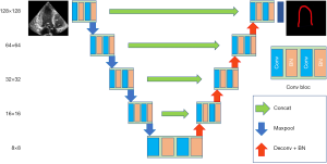
Well-established U-Net neural network architecture proposed by Ronneberger (22) was the first algorithm used in this study. This architecture has been quite successful in biomedical segmentation tasks (11). U-net consists of an encoder performing the contracting and a decoder performing the expansion. Figure 2 illustrates the U-net model used in this study. The model consists of 4 max-pooling layers in the encoder and 4 transposed convolution layers in the decoder. Max-pooling down-samples the images with a 2×2 pooling kernel, 2 strides, and the same-padding method. Similarly, the transposed convolution layer up-samples the images with 4×4 kernel, 2 strides, and the same-padding method. After each transposed convolution layer up-samples the images, same-sized images from the encoder are concatenated to recover fine features, which are lost during the downsampling. All convolution layers use 3×3 kernel, rectified linear unit (ReLU) activation function, and L2 regularization. Batch normalization is used for the normalization scheme. The final convolution layer uses a 1×1 kernel and generates feature maps that have the same number of label classes (3 for our dataset) for prediction. The multi-dimensional dice calculates the loss.
SegAN
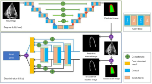
The second algorithm used in this study is the segAN, a neural network architecture for medical image segmentation, proposed by Xue (29). Figure 3 shows the segAN structure. A generative adversarial network model (GAN) consists of a generator (a network that learns how to sample from the underlying distribution of the sample) and discriminator (a network that helps improve the quality of the data-points sampled by the generator). In the segAN architecture, the segmentor (which performs as a generator) produces the predicted segmentation images from original images with encoder-decoder architecture. The critic (which performs as a discriminator) has two inputs, one from the segmentor and the other from the ground truth images, and calculates the loss between two input images. During the training, the segmentor aims to minimize the loss, whereas the critic aims to maximize the same loss. SegAN model is improved while two structures conduct a min-max game. SegAN uses a multi-scale feature loss function based on the mean absolute error (MAE) and dice loss. Xue et al. showed that segAN outperformed other models, including U-net, in the BRATS brain tumor segmentation dataset. After training, segmentor was used for the LV segmentation task. For the segmentor architecture, U-net structure was employed.
Post-processing
Some segmented results from CNNs models made independent island-like structures in the background and an incomplete LV boundary line. Therefore, the post-process was conducted to treat this incompleteness. Morphological Transformation, which is based on the erosion and dilation function (36), was used for our post process. Erosion and dilation combine two sections, respectively, based on the vector subtraction and addition. Erosion, followed by dilation, was used for removing the island structures. Inversely, dilation followed by erosion was used to complete the LV boundary line.
Evaluation of the CNNs models
The performance of the level-set method, which is often used for the automatic segmentation process (37), was calculated on our test dataset to compare the two CNN models with a non-deep learning method. Open-source software was used to apply the level-set method (38). Five images were selected at the same time interval from each of the two pigs in the testing set, a total of 10 images, for each projection to test the level-set method.
For quantitative comparison and assessment of the segmentation results, four widely used metrics in the segmentation research, the dice metric, precision, sensitivity, and Hausdorff distance, were calculated.
Let P and G represent the segmented image and ground truth image, respectively. The dice metric (39) calculates the overlap between P and G, and is defined as:
[1]
The value varies from 0 (no overlap) to 1 (perfect overlap). The higher the value of the dice metric, the better the segmentation. The precision and sensitivity (40) evaluate the relevance of P and G. Precision and sensitivity are defined as follows:
[2]
[3]
where TP, FP, and FN are the numbers of pixels, which are correctly classified as labels, incorrectly classified as labels, and incorrectly classified as not labels in P, respectively. These metrices are normalized (i.e., they vary from 0 to 1). High precision and sensitivity mean that the model makes significantly more relevant results than irrelevant results based on the segmented (P) and ground truth (G) images. The Hausdorff distance (41) calculates the maximum distance between the contours of P(δP) and G(δG). It is defined as:
[4]
where d(i,δ) is the shortest distance from a point i to a contour δ. A low Hausdorff distance value represents a good segmentation result. The unit of the Hausdorff distance is millimeter (mm), which is calculated from information in the echo images.
Statistical analysis
Kruskal-Wallis test was performed for the statistical analysis (42). This test is the non-parametric test and samples do not need to follow the normal distribution. Kruskal-Wallis test assumes that the samples are extracted from the same continuous distribution. P value was calculated using this test and performed as the criteria for the statistical effectiveness.
3D reconstruction
Reconstruction algorithm
3D LV geometries over one cardiac cycle were generated from six standard 2D echo projection images using a 3D reconstruction algorithm developed by our group (31). This algorithm consists of seven steps: endocardium detection, data smoothing, temporal interpolation, sectional scaling and orientation, spatial interpolation, temporal smoothing, and mesh generation. During the sectional scaling and orientation process, six sections are first arranged based on the nominal positions. Next, optimization is conducted by minimizing the difference between the reconstructed and segmented sections.
The dynamic 3D reconstruction algorithm takes six standard-projection delineated videos as the input. One cardiac cycle images, which were generated from the CNN model, were concatenated into a video clip. The size of the output images from CNN models was fixed to 128×128 pixels. Therefore, before concatenating the images, all images were first resized to the original 2D echo image size (e.g., 648×480 pixels) to recover the original LV dimensions. During the 3D reconstruction process, the inner LV boundary of the cavity section was extracted.
Evaluation method or model quantitative assessment
Several LV physiological parameters were calculated based on the pig’s 3D reconstructed volume to evaluate the segmentation results. In this study, reconstructed LV volume with ground truth images is the benchmark volume. Reconstructed LV volume using each CNN models’ segmented images were compared with this benchmark. LV volume was calculated on every time instance during the dynamic 3D reconstruction process. In the reconstruction process, non-dimensional time was used to associate each projection’s different time instances. From one cardiac cycle volume data, EF, stroke volume (SV), and cardiac output (CO) were calculated. These parameters are widely used in cardiac disease diagnosis and perform as the indicators of the LV assessment (43).
The EF is defined as:
[5]
where EDV and ESV are end-diastolic and end-systolic volumes over the given cardiac cycle.
The SV is the difference between the end-diastolic and end-systolic volumes. Finally, CO, i.e., the volume of the blood that is ejected over one minute, is defined as:
[6]
where HR is the heart rate.
Results
Segmentation result
CAMUS dataset segmentation
Two CNN models were tested on the CAMUS dataset to verify the method before employing on the in-house dataset. Additionally, the effect of the post-process, which employed morphological transformation, was calculated on this dataset. Among 450 patients’ images, which are open to the public, 400 patients’ images were assigned to the training set and the rest of (other 50) patients’ images were used for the testing set.
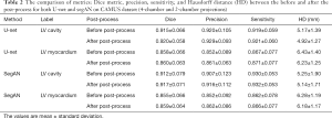
Table 2 reports the dice metric, precision, sensitivity, and Hausdorff distance of U-net and segAN models. Each model’s metric was calculated twice, i.e., before and after the post-processing. The dice metric of the LV cavity is 0.920 for the U-net and 0.917 for the segAN (P value: 0.5617). The dice metric of the LV myocardium is 0.860 for the U-net and 0.859 for the segAN (P value: 0.6068). The precision and sensitivity are evaluated similar to the dice metric. The Hausdorff distance of the LV cavity is 4.92 mm for the U-net and 5.14 mm for the segAN (P value: 0.3992). The Hausdorff distance of the LV myocardium is 6.23 mm for the U-net and 6.18 mm for the segAN (P value: 0.5124). These metrics demonstrate the high performance of both U-net and segAN. However, the difference between U-net and segAN on the metrics was not statistically significant (P value >0.05).
Full table
The effect of the post-process was also calculated on the Table 2. Dice metric increases from 0.915 to 0.920 for the LV cavity (P value: 0.7624) and from 0.858 to 0.860 for the LV myocardium (P value: 0.7457) on the U-net model, and increases from 0.912 to 0.917 for the LV cavity (P value: 0.7216) and from 0.855 to 0.859 for the LV myocardium (P value: 0.6411) on the segAN model.
The Hausdorff distance decreases from 5.17 to 4.92 mm for the LV cavity (P value: 0.1641) and from 6.43 to 6.23 mm for the LV myocardium (P value: 0.0778) on the U-net model, and decreases from 5.25 to 5.14 mm for the LV cavity (P value: 0.7491) and from 6.28 to 6.18 mm for the LV myocardium (P value: 0.4573) on the segAN model. The effect of the post-process stands out on the Hausdorff distance. However, the effect of post-processing was not statistically significant (P value >0.05).
In-house dataset segmentation
U-net and segAN models were trained on the in-house training dataset and tested on the testing dataset for the six standard projections separately. Figure 4 illustrates the original 2D echo images (Gray), predicted segmentation images using the U-net and segAN models (U-net and segAN), ground truth images (Ground Truth), and level-set segmentation images (Level-set) on six standard projections. Green and red regions indicate LV cavity and LV myocardium, respectively, in the U-net, segAN, and ground truth images. The level-set method can only segment the LV cavity which is denoted by a red line in the Level-set images.
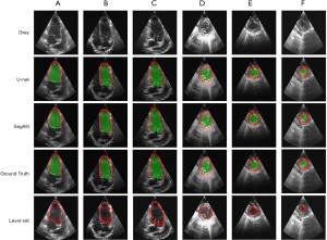
Figure 4 shows that both the U-net and segAN models achieve high performance on LV segmentation. Predicted segmentation images agree with ground truth images converted from expert’s delineation for both the long-axis (Figure 4A,B,C) and short-axis (Figure 4D,E,F) projections. The segmentation difference between U-net and segAN is small and hard to see in the figure.
For the long-axis projections, the level-set method also shows a good agreement with the ground truth in the LV cavity region. However, the existence of valves, which has similar brightness to the LV wall, disturbs the exact segmentation near the base. For the short-axis projections, the presence of the valve orifice, trabeculae, and papillary muscles restricts the LV cavity segmentation. The level-set method generated the curved circular segmentation results for the LV cavity.
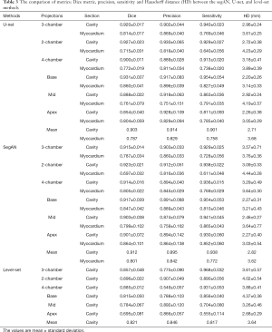
Table 3 shows the dice metric, precision, sensitivity and Hausdorff distance of two CNN models and level-set method calculated on the testing dataset. Metrics of six projections are calculated separately. Mean value of each metric was defined as:
Full table
[7]
where M is each metric (3-chamber: 3ch, 2- and 4-chamber: 2 and 4ch).
The mean dice metric of U-net model is 0.903 for the LV cavity and 0.787 for the LV myocardium. For the LV cavity, the mid and apex projections show smaller dice metric than others (P value: 4.0206×10⁻⁵). For the LV myocardium, the 2-chamber view shows the smallest dice metric value (P value: 4.4151×10⁻⁴).
The mean dice metric of segAN is 0.912 for the LV cavity and 0.801 for the LV myocardium. For the LV cavity, segAN results show similar values for specific projections (P value: 1.3711×10⁻⁴). For the LV myocardium, the 2-chamber view shows the smallest dice metric value (P value: 4.7263×10⁻⁵).
The mean dice metric of the level-set method is 0.821 for the LV cavity and mean Hausdorff distance is 3.64 mm. For the LV cavity, the mid and apex projections show smaller dice metrics than others (P value: 4.1672×10⁻⁸).
From all metrics, U-net and segAN generated better results than the level-set method (P value <0.05). Especially, level-set method showed a lower performance on the short-axis projections than the CNN models. Both U-net and segAN models generated better results on LV cavity than LV myocardium (P value <0.05). The segmentation performance between U-net and segAN is not significant and different with each metrics. For the LV cavity, U-net generated better results on the precision and Hausdorff distance. However, segAN made better results on the dice metric and sensitivity.
Figure 5 shows the final segmentation results. After the resizing process, the LV in Figure 5 has the original height-width ratio and pixel-mm ratio. The videos generated by these images became the input of the 3D reconstruction algorithm. Even though the LV cavity made better segmentation results than LV myocardium, segmented images of LV myocardium were used as the input of the reconstruction algorithm because the reconstruction algorithm only uses the inner boundary of LV.
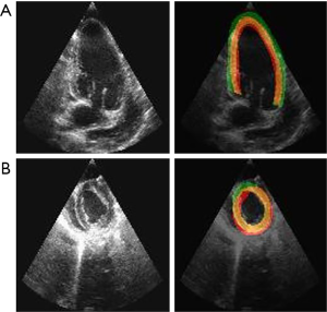
Worst segmentation case
Figure 6 shows the worst segmentation results using CNN models. Both 2-chamber and mid projections’ images were segmented by U-net. The dice metrics of 2-chamber and mid projection images are 0.623 and 0.617, respectively. On the 2-chamber image, segmented LV myocardium (green region) is thicker than the ground truth one. Most of the thicker part is located outside the LV cavity. Left-end part of the segmented myocardium was found to get out of the ground truth more than the right-end. In this case, the CNN model confused the white (bright) part with the myocardium. On the other hand, the segmented LV myocardium of mid projection image was thinner than the ground truth one. Left-upper part of the segmented myocardium was the most deviated part. Here, the CNN model confused the white part as the myocardium again.
3D reconstruction result
Figure 5 shows the first frame images of input videos processed by the dynamic 3D reconstruction algorithm using CNN on segmentation. In this study, the benchmark to evaluate the reconstructed geometries’ physiological parameters was the model reconstructed from ground truth images, which were delineated by experts. Two porcine LV geometries were reconstructed using test dataset images.
Table 4 reports the physiological parameters of reconstructed geometries from the ground truth, U-net segmented, and segAN segmented images. The average error of ejection pressure using the U-net model was 14.0%. The segAN model made 8.4% average error of ejection pressure. For the SV and CO, the U-net model made an average 6.4% error and segAN model made a 10.2% error. These errors are within the 20% error of previous methods using 2D echo compared to the gold standard MRI (44-46). These results showed that the U-net model generated reconstructed volumes, which represented the absolute volume value better than the segAN model. However, the segAN model made LV shapes, which represented the volume trend better than the U-net model.

Full table
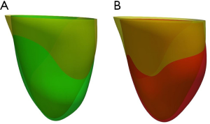
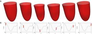
Figure 7 shows the comparison between LV geometries. Yellow LV shape was reconstructed with ground truth images. Red and green LV shapes were reconstructed with segAN and U-net segmented images, respectively. Figure 8 illustrates the 3D reconstruction results over one cardiac cycle generated from segAN segmentation results. Each shape represents the specific time instances with the same time intervals during one cardiac cycle using a fixed apex position and the same point of view. Starting at the end-diastole, the model contracts during the systole and expands during the diastole.
Calculation time
U-net and segAN models were tested using NVIDIA GeForce GTX 1050 GPU. The level-set method was tested on the Intel® Core™ i7-7700HQ CPU. U-net took 53±2 seconds for segmenting the one cardiac cycle images, between 40 to 42 images, i.e., 1.3 seconds per image. The segAN model required average 104±8 seconds to segment the one cardiac cycle images, i.e., 2.51 seconds per image. The level-set method took 75±2 seconds for segmenting one image.
3D reconstruction algorithm was operated on the Intel Xeon E5-2670 v2 CPU. It required approximately 49 seconds to reconstruct the geometry of one cardiac cycle.
Segmentation of the six projection images over one cardiac cycle and 3D reconstruction using U-net required 367 seconds on average.
Discussion
In-house dataset analysis
Our in-house dataset is different from the datasets previously available for segmentation of LV in 2D echo. The previous datasets only consisted of one- or two-time instants, e.g., end-diastolic and end-systolic images, from each case. Those datasets had 60 to 450 different cases to support data diversity (4,24,25). However, our in-house dataset consisted of 30 to 40 images from one case and had 10 different cases. The segmentation results showed that, if the total number of images is enough, our new kind of dataset also achieves a high performance on the segmentation task. However, due to the small number of cases, the limitation of the current segmentation model is that it only worked well on similar 2D echo images, which are obtained from the same transducer. This problem can be solved by increasing the number of cases.
In the current study, six standard projections were trained individually based on in-house dataset. There is a clear structure difference, such as the number of chambers in long-axis projections, between six standard projections which are captured during the 2D echo image acquisition process. Therefore, each projection’s images have similar arrangement of structures and shape of cardiac structures. For this reason, training individual projections showed a higher segmentation performance than training with all projections together. For example, base projection’s LV cavity segmentation showed that the U-net model, which was trained on the base, mid, and apex images, generated 0.872 dice metric and 2.41 mm Hausdorff distance, whereas training with only the base images generated 0.931 Dice metric and 2.20 mm Hausdorff distance.
Our segmentation results show that the usage of 2D echo images can be extended with CNN models by removing segmentation restrictions. Currently, CNN models are actively used in the segmentation of MRI and CT cardiac images (15). Most of the LV MRI and CT datasets consist of dense short-axis images. CNN models achieve more than 0.9 on the dice loss and precision for these image segmentation task (17-19). Our study shows that the CNN models also can achieve a similar accuracy on 2D echo projections. It suggests that if there is a large dataset for the segmentation, the data types, e.g., MRI, CT and echo, would not significantly affect the performance of the CNN models.
Post-process analysis
CNN models’ segmented results showed some unexpected island-like structures in the background. The post-process followed the segmentation task to remove these island-like structures. The island-like structures caused a higher Hausdorff distance, which calculates the maximum distance between two contours, because most of the island-like structures were located on the edge of the background. However, the dice metric, precision, and sensitivity did not decrease a lot, because they occupied a small number of pixels compared to all of pixels of the LV cavity and myocardium. Table 2 represents the effect of the post-process. Comparing the metrics before and after conducting the post-processing, the Hausdorff distance was decreased around 1.4% to 4.7%, while other metrics increased less than 1%. However, the metrices of LV myocardium were still worse than LV cavity’s metrics after post-processing. There are two main reasons for such lower metric values. First, the total number of pixels were inherently different between the LV cavity and myocardium. LV cavity had a larger number of pixels which is advantageous for calculating the metrics. Second, current post-process method removed the isolated part whose diameter is less than the input value. This input value was chosen to be less than the LV myocardium thickness, because the segmented LV myocardium should not be affected by the post-process. For this reason, the island-like structures whose diameters were larger than the LV myocardium thickness were not removed by the current post-processing. Other background removing methods, such as the region of interest technique, should be developed to increase the segmentation accuracy.
Comparing U-net, segAN, and level-set methods
Figure 9 shows the comparison between the U-net and segAN models using the Tukey box of dice metric results. From these plots, U-net outperformed the segAN for the 2-chamber and base projections. In contrast, for the apex projection, segAN performed better than the U-net. For the other three projections, the superiority of one model is not clear. Based on the segmentation time, the segAN took twice time than the U-net on the same GPU.
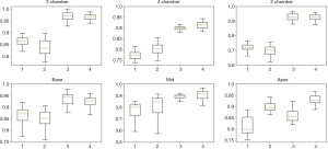
Table 3 shows that the U-net and segAN models outperformed the level-set method on the LV segmentation task for the 2D echo images. The level-set method caused several specific problems. For the long-axis, the aortic and mitral valves, which were located between the LV and left atrium, disturbed the exact LV cavity segmentation. The seriousness of this problem changed over the cardiac cycle with opening and closing of the valves. The worst-case occurred when the valve was open. The level-set method could not distinguish between the LV and the left atrium. To get a reasonable breakpoint between the two structures, the total number of iterations should be carefully controlled by experts for the level-set, i.e., not fully automatic. For the short-axis, the existence of trabeculae and papillary muscle, which had similar brightness on 2D echo images, caused distorted segmentation results. However, CNN models generated segmentation results regardless of these problems on both long- and short-axis images. Furthermore, the CNN techniques were fully automatic. In contrast, the level-set method needed a manual starting box, which should be chosen carefully. Finally, the level-set method spent more calculation time than the machine learning models. The level-set method took almost 50 minutes to segment the images for one cardiac cycle.
Limitations
To make up for the insufficient datasets, transfer learning and augmentation techniques were employed. However, the different quality of the 2D echo images, e.g., sparse borders, variation in echo, and image noise, restricted the application of the trained models. When the model tries to segment different quality images, it generates non-robust segmentation results with incomplete segmentation lines and large island-like structures. Also, some 2D echo images depict cavities other than the LV. These limitations could be improved by training with a larger and diverse dataset.
The in-house dataset was obtained from open-chest pigs. As mentioned in the methods section, pig's cardiovascular anatomy closely replicates human cardiovascular anatomy and physiology (32) and open-chest is preferred as it allows reproduction of standardized echocardiographic projections which is not possible in closed-chest due to differences in chest configuration and intercostal space between pigs and humans (33). Open-chest echocardiographic scans do not include signal loss (attenuation) that would otherwise be caused by soft tissues within an intercostal imaging window during human transthoracic echocardiography. The avoided signal loss is generally an advantage because attenuation artifacts do not compromise the experimental scans’ quality, i.e., open-chest porcine echo has better quality than human echo. Nevertheless, we have shown that the method works on humans using the CAMUS dataset. In addition, the method was pre-trained (transfer learning) using the CAMAS dataset for two of the standard cross-sections (long-axis). Therefore, the methods used in this study can also be applied to humans.
Future work
For the future work, the automatic delineation method needs to be extended to segment the valves, which is not a trivial task because only small numbers of pixels represent the valves in standard 2D echo projections thus making it hard to distinguish them from LV ends in long-axis and tendineae in short-axis projections. Nevertheless, such capability enables creating a closed geometry that can be used for image-based computational fluid dynamics (CFD) simulations (47,48) and fluid-structure interaction simulations (49).
Here, we have used several pigs for training and testing. The study is designed to facilitate the translation to clinical data by using standard cross-sections for echo acquisition. In fact, we showed the method could successfully segment the human echo data in CAMUS dataset. Nevertheless, the application of the method to real clinical data is left for future.
Conclusions
In this study, a dynamic 3D LV model is automatically generated from six standard gray-scale 2D echo images. This process consists of automatic segmentation of the 2D echo images followed by 3D reconstruction of the segments. The deep learning (CNN) segmentation method facilitates a more rapid and consistent 3D reconstruction model from 2D echo images.
Two CNN models, U-net and segAN, have been employed to segment the LV from 2D echo images automatically. We trained the CNN models with an in-house dataset, which uniquely consisted of three long-axis and three short-axis LV projections over one cardiac cycle. Transfer learning with a CAMUS dataset (for two of long-axis projections) and augmentation methods were used to compensate for a relatively small amount of training data.
The assessment metrics and segmented images show that both U-net and segAN achieve high performance on LV segmentation. U-net mean average 0.903 and 0.787 dice metrics for the LV cavity and myocardium, respectively. SegAN achieved mean 0.912 and 0.801 dice metrics for the LV cavity and myocardium, respectively. In addition, segmentation results were evaluated by using a dynamic 3D reconstruction algorithm.
A fully automated pipeline, from 2D echo images to a 3D geometric geometry of LV, was generated by combining the machine learning segmentation technique and a 3D reconstruction algorithm. This pipeline can help the rapid and hi-fidelity analysis of echo images in clinical applications to visualize 3D LV wall motion and evaluate global function. Our methodology offers a new direction in patient-specific LV modeling and simulation to augment the experts’ effort and simultaneously enhance the accuracy of their analysis
Acknowledgments
Funding: This work was supported by the Texas A&M High Performance Research Computing center (HPRC). The animal studies were supported by the NIH R01 grant EB019947.
Footnote
Conflicts of Interest: All authors have completed the ICMJE uniform disclosure form (available at http://dx.doi.org/10.21037/qims-20-745). Dr. MB reports grants from National Institutes of Health, during the conduct of the study. The other authors have no conflicts of interest to declare.
Ethical Statement: The Institutional Animal Care and Use Committee of the Mayo Clinic approved the research protocol, in compliance with the national guidelines, the Guide for the Care and Use of Laboratory Animals, 8th Edition, 2011. The animal care program for the Mayo Clinic Arizona campus, where the studies were conducted, is AAALAC accredited and has an approved Animal Welfare Assurance through the Office of Laboratory Animal Welfare (OLAW).
Open Access Statement: This is an Open Access article distributed in accordance with the Creative Commons Attribution-NonCommercial-NoDerivs 4.0 International License (CC BY-NC-ND 4.0), which permits the non-commercial replication and distribution of the article with the strict proviso that no changes or edits are made and the original work is properly cited (including links to both the formal publication through the relevant DOI and the license). See: https://creativecommons.org/licenses/by-nc-nd/4.0/.
References
- Lang RM, Badano LP, Tsang W, Adams DH, Agricola E, Buck T, Faletra FF, Franke A, Hung J, de Isla LP, Kamp O, Kasprzak JD, Lancellotti P, Marwick TH, McCulloch ML, Monaghan MJ, Nihoyannopoulos P, Pandian NG, Pellikka PA, Pepi M, Roberson DA, Shernan SK, Shirali GS, Sugeng L, Ten Cate FJ, Vannan MA, Zamorano JL, Zoghbi WA. EAE/ASE recommendations for image acquisition and display using three-dimensional echocardiography. Eur Heart J Cardiovasc Imaging 2012;13:1-46. [Crossref] [PubMed]
- Yodwut C, Weinert L, Klas B, Lang RM, Mor-Avi V. Effects of frame rate on three-dimensional speckle-tracking-based measurements of myocardial deformation. J Am Soc Echocardiogr 2012;25:978-85. [Crossref] [PubMed]
- Porshnev S, Bobkova A, Zyuzin V, Bobkov VJ Fr. Method of semi-automatic delineation of the left ventricle of the human heart on echographic images. Fundamental research 2013;8:44-8.
- Leclerc S, Smistad E, Pedrosa J, Ostvik A, Cervenansky F, Espinosa F, Espeland T, Berg EAR, Jodoin PM, Grenier T, Lartizien C, Dhooge J, Lovstakken L, Bernard O. Deep Learning for Segmentation Using an Open Large-Scale Dataset in 2D Echocardiography. IEEE Trans Med Imaging 2019;38:2198-210. [Crossref] [PubMed]
- Cocosco CA, Niessen WJ, Netsch T, Vonken EJ, Lund G, Stork A, Viergever MA. Automatic image-driven segmentation of the ventricles in cardiac cine MRI. J Magn Reson Imaging 2008;28:366-74. [Crossref] [PubMed]
- Liu H, Hu H, Xu X, Song E. Automatic left ventricle segmentation in cardiac MRI using topological stable-state thresholding and region restricted dynamic programming. Acad Radiol 2012;19:723-31. [Crossref] [PubMed]
- Billet F, Sermesant M, Delingette H, Ayache N. editors. Cardiac motion recovery and boundary conditions estimation by coupling an electromechanical model and cine-MRI data. International Conference on Functional Imaging and Modeling of the Heart; 2009: Springer.
- Zhang H, Wahle A, Johnson RK, Scholz TD, Sonka M. 4-D cardiac MR image analysis: left and right ventricular morphology and function. IEEE Trans Med Imaging 2010;29:350-64. [Crossref] [PubMed]
- Zhuang X, Hawkes DJ, Crum WR, Boubertakh R, Uribe S, Atkinson D, Batchelor P, Schaeffter T, Razavi R, Hill DL. editors. Robust registration between cardiac MRI images and atlas for segmentation propagation. Medical Imaging 2008: Image Processing; 2008: International Society for Optics and Photonics.
- Petitjean C, Dacher JN. A review of segmentation methods in short axis cardiac MR images. Med Image Anal 2011;15:169-84. [Crossref] [PubMed]
- Litjens G, Kooi T, Bejnordi BE, Setio AAA, Ciompi F, Ghafoorian M, van der Laak J, van Ginneken B, Sanchez CI. A survey on deep learning in medical image analysis. Med Image Anal 2017;42:60-88. [Crossref] [PubMed]
- de Vos BD, Wolterink JM, Leiner T, de Jong PA, Lessmann N, Isgum I. Direct Automatic Coronary Calcium Scoring in Cardiac and Chest CT. IEEE Trans Med Imaging 2019;38:2127-38. [Crossref] [PubMed]
- Ciompi F, de Hoop B, van Riel SJ, Chung K, Scholten ET, Oudkerk M, de Jong PA, Prokop M, van Ginneken BJ. Automatic classification of pulmonary peri-fissural nodules in computed tomography using an ensemble of 2D views and a convolutional neural network out-of-the-box. Med Image Anal 2015;26:195-202. [Crossref] [PubMed]
- Wolterink JM, Leiner T, de Vos BD, van Hamersvelt RW, Viergever MA, Isgum I. Automatic coronary artery calcium scoring in cardiac CT angiography using paired convolutional neural networks. Med Image Anal 2016;34:123-36. [Crossref] [PubMed]
- Gardner BI, Bingham SE, Allen MR, Blatter DD, Anderson JL. Cardiac magnetic resonance versus transthoracic echocardiography for the assessment of cardiac volumes and regional function after myocardial infarction: an intrasubject comparison using simultaneous intrasubject recordings. Cardiovasc Ultrasound 2009;7:38. [Crossref] [PubMed]
- Suinesiaputra A, Cowan BR, Al-Agamy AO, Elattar MA, Ayache N, Fahmy AS, Khalifa AM, Medrano-Gracia P, Jolly MP, Kadish AH, Lee DC, Margeta J, Warfield SK, Young AA. A collaborative resource to build consensus for automated left ventricular segmentation of cardiac MR images. Med Image Anal 2014;18:50-62. [Crossref] [PubMed]
- Bernard O, Lalande A, Zotti C, Cervenansky F, Yang X, Heng PA, Cetin I, Lekadir K, Camara O, Gonzalez Ballester MA, Sanroma G, Napel S, Petersen S, Tziritas G, Grinias E, Khened M, Kollerathu VA, Krishnamurthi G, Rohe MM, Pennec X, Sermesant M, Isensee F, Jager P, Maier-Hein KH, Full PM, Wolf I, Engelhardt S, Baumgartner CF, Koch LM, Wolterink JM, Isgum I, Jang Y, Hong Y, Patravali J, Jain S, Humbert O, Jodoin PM. Deep Learning Techniques for Automatic MRI Cardiac Multi-Structures Segmentation and Diagnosis: Is the Problem Solved? IEEE Trans Med Imaging 2018;37:2514-25. [Crossref] [PubMed]
- Bai W, Sinclair M, Tarroni G, Oktay O, Rajchl M, Vaillant G, Lee AM, Aung N, Lukaschuk E, Sanghvi MM, Zemrak F, Fung K, Paiva JM, Carapella V, Kim YJ, Suzuki H, Kainz B, Matthews PM, Petersen SE, Piechnik SK, Neubauer S, Glocker B, Rueckert D. Automated cardiovascular magnetic resonance image analysis with fully convolutional networks. J Cardiovasc Magn Reson 2018;20:65. [Crossref] [PubMed]
- Zreik M, Leiner T, De Vos BD, van Hamersvelt RW, Viergever MA, Išgum I. editors. Automatic segmentation of the left ventricle in cardiac CT angiography using convolutional neural networks. 2016 IEEE 13th International Symposium on Biomedical Imaging (ISBI); 2016: IEEE.
- Lieman-Sifry J, Le M, Lau F, Sall S, Golden D. editors. FastVentricle: cardiac segmentation with ENet. International Conference on Functional Imaging and Modeling of the Heart; 2017: Springer.
- Çiçek Ö, Abdulkadir A, Lienkamp SS, Brox T, Ronneberger O. editors. 3D U-Net: learning dense volumetric segmentation from sparse annotation. International conference on medical image computing and computer-assisted intervention; 2016: Springer.
- Ronneberger O, Fischer P, Brox T. editors. U-net: Convolutional networks for biomedical image segmentation. International Conference on Medical image computing and computer-assisted intervention; 2015: Springer.
- Tan LK, Liew YM, Lim E, McLaughlin RA. Convolutional neural network regression for short-axis left ventricle segmentation in cardiac cine MR sequences. Med Image Anal 2017;39:78-86. [Crossref] [PubMed]
- Veni G, Moradi M, Bulu H, Narayan G, Syeda-Mahmood T. editors. Echocardiography segmentation based on a shape-guided deformable model driven by a fully convolutional network prior. 2018 IEEE 15th International Symposium on Biomedical Imaging (ISBI 2018); 2018: IEEE.
- Zhang J, Gajjala S, Agrawal P, Tison GH, Hallock LA, Beussink-Nelson L, Lassen MH, Fan E, Aras MA, Jordan C, Fleischmann KE, Melisko M, Qasim A, Shah SJ, Bajcsy R, Deo RC. Fully Automated Echocardiogram Interpretation in Clinical Practice. Circulation 2018;138:1623-35. [Crossref] [PubMed]
- Li M, Zhang W, Yang G, Wang C, Zhang H, Liu H, Zheng W, Li S. editors. Recurrent aggregation learning for multi-view echocardiographic sequences segmentation. International Conference on Medical Image Computing and Computer-Assisted Intervention; 2019: Springer.
- Li M, Wang C, Zhang H, Yang G. MV-RAN: Multiview recurrent aggregation network for echocardiographic sequences segmentation and full cardiac cycle analysis. Comput Biol Med 2020.103728. [Crossref] [PubMed]
- Lang RM, Bierig M, Devereux RB, Flachskampf FA, Foster E, Pellikka PA, Picard MH, Roman MJ, Seward J, Shanewise J, Solomon S, Spencer KT, St John Sutton M, Stewart W. Recommendations for chamber quantification. Eur J Echocardiogr 2006;7:79-108. [Crossref] [PubMed]
- Xue Y, Xu T, Zhang H, Long LR, Huang X, Seg AN. Adversarial Network with Multi-scale L1 Loss for Medical Image Segmentation. Neuroinformatics 2018;16:383-92. [Crossref] [PubMed]
- Chukwu EO, Barasch E, Mihalatos DG, Katz A, Lachmann J, Han J, Reichek N, Gopal AS. Relative importance of errors in left ventricular quantitation by two-dimensional echocardiography: insights from three-dimensional echocardiography and cardiac magnetic resonance imaging. J Am Soc Echocardiogr 2008;21:990-7. [Crossref] [PubMed]
- Rajan NK, Song Z, Hoffmann KR, Belohlavek M, McMahon EM, Borazjani I. Automated Three-Dimensional Reconstruction of the Left Ventricle From Multiple-Axis Echocardiography. J Biomech Eng 2016. [Crossref] [PubMed]
- Crick SJ, Sheppard MN, Ho SY, Gebstein L, Anderson RH. Anatomy of the pig heart: comparisons with normal human cardiac structure. J Anat 1998;193:105-19. [Crossref] [PubMed]
- Kerut EK, Valina CM, Luka T, Pinkernell K, Delafontaine P, Alt EU. Technique and imaging for transthoracic echocardiography of the laboratory pig. Echocardiography 2004;21:439-42. [Crossref] [PubMed]
- Manovel A, Dawson D, Smith B, Nihoyannopoulos P. Assessment of left ventricular function by different speckle-tracking software. Eur J Echocardiogr 2010;11:417-21. [Crossref] [PubMed]
- Bagger T, Sloth E, Jakobsen CJ. Left ventricular longitudinal function assessed by speckle tracking ultrasound from a single apical imaging plane. Crit Care Res Pract 2012;2012:361824. [Crossref] [PubMed]
- Haralick RM, Sternberg SR, Zhuang X. Image analysis using mathematical morphology. IEEE Trans Pattern Anal Mach Intell 1987;9:532-50. [Crossref] [PubMed]
- Li C, Xu C, Gui C, Fox MD. Distance regularized level set evolution and its application to image segmentation. IEEE Trans Image Process 2010;19:3243-54. [Crossref] [PubMed]
- Dietenbeck T, Alessandrini M, Friboulet D, Bernard O. editors. CREASEG: a free software for the evaluation of image segmentation algorithms based on level-set. 2010 IEEE International Conference on Image Processing; 2010: IEEE.
- Dice LR. Measures of the amount of ecologic association between species. Ecology 1945;26:297-302. [Crossref]
- Powers DM. Evaluation: from precision, recall and F-measure to ROC, informedness, markedness and correlation. J Mach Learn Technol 2011;2:37-63.
- Huttenlocher DP, Klanderman GA, Rucklidge WJ. Comparing images using the Hausdorff distance. 1992 IEEE Computer Society Conference on Computer Vision and Pattern Recognition 1993;15:850-63.
- Kruskal WH, Wallis WA. Use of ranks in one-criterion variance analysis. J Am Stat Assoc 1952;47:583-621. [Crossref]
- Reiter U, Reiter G, Manninger M, Adelsmayr G, Schipke J, Alogna A, Rajces A, Stalder AF, Greiser A, Muhlfeld C, Scherr D, Post H, Pieske B, Fuchsjager M. Early-stage heart failure with preserved ejection fraction in the pig: a cardiovascular magnetic resonance study. J Cardiovasc Magn Reson 2016;18:63. [Crossref] [PubMed]
- Hoffmann R, Barletta G, von Bardeleben S, Vanoverschelde JL, Kasprzak J, Greis C, Becher HJ. Analysis of left ventricular volumes and function: a multicenter comparison of cardiac magnetic resonance imaging, cine ventriculography, and unenhanced and contrast-enhanced two-dimensional and three-dimensional echocardiography. J Am Soc Echocardiogr 2014;27:292-301. [Crossref] [PubMed]
- Greupner J, Zimmermann E, Grohmann A, Dübel HP, Althoff T, Borges AC, Rutsch W, Schlattmann P, Hamm B, Dewey MJ. Head-to-head comparison of left ventricular function assessment with 64-row computed tomography, biplane left cineventriculography, and both 2- and 3-dimensional transthoracic echocardiography: comparison with magnetic resonance imaging as the reference standard. J Am Coll Cardiol 2012;59:1897-907. [Crossref] [PubMed]
- Hoffmann R, von Bardeleben S, ten Cate F, Borges AC, Kasprzak J, Firschke C, Lafitte S, Al-Saadi N, Kuntz-Hehner S, Engelhardt MJ. Assessment of systolic left ventricular function: a multi-centre comparison of cineventriculography, cardiac magnetic resonance imaging, unenhanced and contrast-enhanced echocardiography. Eur Heart J 2005;26:607-16. [Crossref] [PubMed]
- Hedayat M, Patel TR, Kim T, Belohlavek M, Hoffmann KR, Borazjani I. A hybrid echocardiography‐CFD framework for ventricular flow simulations. Int J Numer Method Biomed Eng 2020;36:e03352. [Crossref] [PubMed]
- Borazjani I, Westerdale J, McMahon EM, Rajaraman PK, Heys JJ, Belohlavek M. Left ventricular flow analysis: recent advances in numerical methods and applications in cardiac ultrasound. Comput Math Methods Med 2013;2013:395081. [Crossref] [PubMed]
- Borazjani I. A review of fluid-structure interaction simulations of prosthetic heart valves. J Long Term Eff Med Implants 2015;25:75-93. [Crossref] [PubMed]


