A fully automated left atrium segmentation approach from late gadolinium enhanced magnetic resonance imaging based on a convolutional neural network

Introduction

Atrial fibrillation (AF) is the most common arrhythmia in the western world with an incidence of about 0.4% in men and 0.6% in women. It is known that the prevalence of AF in US is about 2.2 million including paroxysmal or persistent AF (1). Moreover, about 160,000 new AF cases each year only in the US and in the European countries are diagnosed. Consequences of AF could lead to a notable reduction in quality of life, poor mental health, disability, dementia and, mainly, an increase of stroke risk by five-fold (2).

Radio frequency ablation (RFA) of the left atrium (LA) represents the clinical therapy for AF patients in which antiarrhythmic drugs and direct current cardioversion do not provide improvements for patient’s health. Haissaguerre and colleagues identified the pulmonary veins (PVs) as the most common sites for AF triggers (3); for this reason, PV isolation (PVI) has become the milestone of AF RFA. However, despite strong improvements for the targeting and the delivery of AF RFA, the long-term restoration of sinus rhythm is achieved only in a limited percentage of AF patients: AF-free rates after a single ablation vary between 30% and 50% at 5 years follow-up (4,5). These results suggest there is room for improvements in RFA treatment and underline a lack of understanding of mechanisms sustaining AF.

Magnetic resonance imaging (MRI) is capable of differentiating between scarred and non-scarred atrial wall by using late gadolinium enhancement (LGE) imaging. Several clinical studies suggested that LA fibrosis is associated with AF and with AF recurrence after ablation (6). LGE MRI allows the detection of the fibrotic tissue to identify native and post-ablation atrial scarring leading to an improvement of the success rate of the RFA (7-9). Unfortunately, in clinical practice, LGE MRI is rarely considered since a standard acquisition protocol is not available (10). Electro-anatomical voltage maps are used during RFA as a surrogate index of fibrosis, by considering low voltage regions corresponding to fibrotic tissue areas (7). In addition, even if studies on atrial structure segmentation applied to LGE MRI have shown promising results, most of them were based on a time-consuming procedure of manual tracing of LA wall and PVs (8,11-13). Results are affected by high variability among experts and low reproducibility in multicenter studies.

Different approaches for LA segmentation have been proposed but they are based on different MRI data. Valinoti et al. (14) proposed a 3-D LA patient-specific model from MRI angiography acquired in 26 patients; the anatomical model could be easily integrated with fibrosis information from LGE MRI by simply registering the two datasets and using grey-level intensities from LGE MRI as a texture of the 3-D anatomical model. Similarly, Yang et al. (15) proposed a combined pipeline involving a multi-atlas-based whole heart segmentation to determine cardiac anatomy from a balanced steady state free precession sequence which was then mapped to LGE MRI. Their approach was tested on data from 37 patients. Only very few studies were recently proposed to segment LA chamber directly from LGE MRI. Tao et al. (16) developed a fully automatic method for LA and PVs segmentation, with comparable performance to a human observer. Their approach was tested on data from 46 patients; unfortunately, it requires substantial computation time due to the multi-atlas-based registration. Recently, deep learning techniques were largely used for MRI data processing (17,18), showing a growing interest in the design of MRI detection, classification, reconstruction and segmentation algorithms. This was also confirmed during the Statistical Atlases and Computational Modelling of the Heart (STACOM) 2018 Atrial Segmentation Challenge, focused on automatic LA segmentation from LGE MRI. Most of the proposed approaches were based on Convolutional Neural Networks (CNNs), adopting 2-D (17) or 3-D (19,20) architectures. The winning solution (18) makes use of a double 3-D CNN, localizing the target region in the first CNN and producing a fine segmentation in the second CNN. Despite the promising results obtained in this challenge, it is not clear how a 3-D pipeline affects the output segmentation at the level of the LA regions where the cross-subject variability is high (e.g., regions near the mitral valve and the PVs). In addition, the high computational cost related to a CNN-based LA localization (first stage of the double CNN approach) limits its applicability in a clinical scenario. Very recently, Xiong et al. (21) proposed AtriaNet, a multi-scale dual pathway 2-D CNN able to capture both LA local and global information; AtriaNet was trained and tested on LGE MRI data from the STACOM 2018 Atrial Segmentation Challenge and showed very accurate results using 2-D axial patches of different size extracted from 3-D LGE MRI data. The architecture proposed (21) is quite complex, involving a large amount of trainable parameters (15,448,896), and requires a large number of cardiac data for training as well as an extensive hyper-parameter tuning procedure to optimize segmentation results due to the less clear setting of the new hyper-parameters introduced (e.g., input patch size of the local and global pathways).

The aim of this study was to design and test a simple and lightweight fully automatic pipeline for LA segmentation from LGE MRI. The proposed approach was tested on 3-D data using as input the 2-D slices or the 3-D volume to provide a direct comparison between different approaches. This comparison was further extended to three LA sub volumes (near the mitral valve, central, containing the PVs) to evaluate the differential behavior of the two pipelines along the LA longitudinal extension.

Methods

Dataset

The deepened pipelines were developed on the STACOM 2018 Atrial Segmentation Challenge dataset, which includes 154 LGE MRI 3-D cardiac images. Only 100 out of 154 images were provided for the challenge and made available (http://atriaseg2018.cardiacatlas.org) with the related 3-D ground truth segmentations (0 for background and 1 for LA) and the organizers during the competition provided the results on the 54 test set images. Since the 54 test images were not labeled, this study was conducted only on the 100 labeled cardiac images. In the following, the tuple composed by a 3-D cardiac image and the related ground truth segmentation is named as cardiac data. The data resolution was 0.625×0.625×0.625 mm³ and the 3-D cardiac data was composed by 88 axial slices with in-plane size of 576×576 or 640×640 pixels. To train the CNN in the two proposed approaches, the dataset was randomly split into a training set (80%, 80 cardiac data) and a test set (20%, 20 cardiac data). To perform early stopping in the first training run, a validation set of 10% (8 cardiac data) of the training set was selected.

Data used in this study have obtained ethics approval in the respective Institutions in which they were acquired before their use for the STACOM 2018 Atrial Segmentation Challenge dataset and are freely available under request (http://atriaseg2018.cardiacatlas.org).

Stage I: Left atrium localization via Otsu’s algorithm

LGE MRI images are acquired in the axial plane using a standard protocol in which the LA chamber is located in the center of the images. This information can be exploited in order to facilitate the following analysis aimed at fine segmentation. Furthermore, it is functional to reduce the number of pixels or voxels from which the CNN extracts information, and therefore the computational cost of the CNN training. The subject specific LA position was automatically assessed by applying a rough LA segmentation based on Otsu’s algorithm to the central axial slice of each 3-D cardiac image (Figure 1). Once the binary image resulting from Otsu’s segmentation was obtained, the bounding box around the central region was automatically computed (green box in Figure 1B). Then, the size of the bounding box was increased to 320×384 pixel and a 3-D crop of fixed size 88×320×384 was extracted (yellow box, Figure 1B,C). This procedure allowed the correct crop of the LA region in all LGE MRI data.

Figure 1 Results of the rough segmentation and pre-processing. The middle axial slice of an illustrative input image (A) was roughly segmented using Otsu’s algorithm (B). After labeling the bounding box around the bigger central region was computed (B, green box). The size of the bounding box was then increased (B, yellow box) and, finally, the crop containing the LA was extracted (C). LA, left atrium.

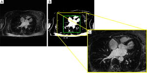
Data were then subsampled to 88×192×240 for the 2-D pipeline and to 80×192×240 for the 3-D pipeline. This last resizing of the images along the third dimension (from 88 to 80) allowed a match between the dimensions of the tensors in the concatenation layers of the CNN in the 3-D approach. These subsampled crops containing LA were used for the training, and all the tissues outside this crop were classified as background.

The CNN was trained with these subsampled cardiac data with 2-D axial slices extracted from the cardiac data in the 2-D pipeline and with the 3-D volumes in the 3-D pipeline. In the 2-D pipeline the number of training, test and validation examples was 6,336, 1,760, 704, respectively, while in the 3-D pipeline was 72, 20, 8, respectively.

Stage II: Fine segmentation via 2-D or 3-D CNN

In the following the architecture of the CNN, the training process, the inference and post-processing steps, and the evaluation metric are described.

CNN architecture

The deep learning approach proposed for the 2-D and 3-D pipelines was based on the successful U-Net architecture (Figure 2). The main hyper-parameters were chosen following the original U-Net architecture, while the number of convolutional filters and the learning rate were chosen empirically during an early manual hyper-parameter evaluation stage. In the convolutional layers, kernel size of 3×3×3 (3-D approach) or 3×3 (2-D approach), stride size of 1×1×1 or 1×1 and Rectified Linear Units (ReLUs) activation functions in the hidden layers or sigmoidal activation function in the output layer were used. In the max pooling layers, a pooling size of 2×2×2 or 2×2 and stride size of 2×2×2 or 2×2, halving the shape of hidden activations, were employed. Lastly, in the transposed convolutional layers, kernel size of 2×2×2 or 2×2 and stride size of 2×2×2 or 2×2 were applied. For both convolutional and transposed convolutional layers, padding size was such that the output shape of the layer was the same of the input shape. Furthermore, biases and weights were randomly initialized from a truncated normal distribution and using the initialization scheme proposed by He et al. (22) for ReLUs, respectively.

Figure 2 The adopted 3-D CNN architecture. Each box specifies the tensor shape for each of the layers of the CNN and the arrow colors encode different operators as explained in the legend. The two gray boxes represent the input and output tensors, the blue boxes the outputs of the convolutional layers, the red boxes the max pooled activations and the green boxes the concatenation between the activations of the transposed convolutional layers and the corresponding activations in the encoder module. The 2-D architecture shared the same hyper-parameters and can be easily obtainable from the 3-D architecture. CNN, convolutional neural network.

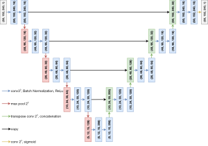
In addition to the original version of the U-Net (23), after each convolutional layer and before the activation function, a batch normalization layer (24) was included. This is an adaptive reparameterization technique introduced to reduce the covariance shift and to speed up the training process making models less sensitive to the parameter’s initialization. Furthermore, it introduces a regularization effect and, sometimes, reduces the need of computationally heavy regularizers (22), such as Dropout (25).

The overall number of parameters for the 2-D approach was 1,946,705 (1,943,761 trainable parameters), while for the 3-D approach it was 5,650,801 (5,647,857 trainable parameters).

Training process

The CNN training was driven by a Soft-Dice loss function (26) proposed to introduce a balancing between foreground and background voxels (or pixels in the 2-D approach).

The Soft-Dice coefficient (SDC) is an extension of the Dice coefficient that relies on the concept of disagreement between pairs of probabilistic classifications (27). Given the segmentation S and the ground truth G, the classes S_i and G_i of the i-th voxel can be defined as random variables on the label space {0,1}. The probabilistic segmentations can be represented as label probability maps: p={p_i:=P(S_i=1)} and g={g_i:=P(G_i=1)}. In our case, the ground truth probability map g is such that $g_i\in \left\{0,1\right\}\forall \text{i}$ and the associated SDC can be written as {see Equation [1]}:

$$SDC\left(p,q\right)=\frac{2{{\displaystyle \sum }}_{i=1}^N{p}_i{g}_i}{{{\displaystyle \sum }}_{i=1}^N\left(p_i+g_i\right)}$$[1]

where the sums run over the N voxels (or pixels) of the predicted 3-D (or 2-D) probability map p and the corresponding ground truth probability map g.

When dealing with medical images it is common that the anatomy to segment occupies small regions of the image. This can cause a strong bias towards the background during the CNN training and thus the foreground regions in the resulting predicted segmentations are often under-represented or missing. To solve this strong class unbalancing, a viable solution consists in a weighted loss function in which a sample re-weighting is included, giving more importance to the foreground regions with respect to the background regions during the training of the CNN (26). Another solution proposed by Milletari et al. (26) and used in this work consists in the optimization of the Soft-Dice loss function based on a different formulation of the SDC. This solution removes the need to assign weights to samples to get the right class balance, leading to better experimental results than the ones obtained with the sample re-weighting approach. Thus, the SDC formulation {see Equation [1]} was modified see Equation [2] (26):

$$SDC\left(p,q\right)=\frac{2{{\displaystyle \sum }}_{i=1}^N{p}_i{g}_i}{{{\displaystyle \sum }}_{i=1}^N\left(p_i{}^2+g_i{}^2\right)}$$[2]

where the sums run over the N voxels (or pixels) of the predicted 3-D (or 2-D) probability map p and the corresponding ground truth probability map g.

Then, the Soft-Dice loss function was computed as Equation [3]:

$$SDloss\left(p,q\right)=1-SDC\left(p,q\right)$$[3]

The ADAM optimizer (28) was employed with exponential decay rates β₁=0.9, β₂=0.999. The learning rate ε was 1e-3 and a batch size of 32 and 2 was used for the 2-D and 3-D approaches, respectively.

The training process was subdivided into two runs, as proposed in (29). In the first run early stop was performed (30) and thus, the CNN was trained until the validation loss (SD loss computed on 704 samples in 2-D and on 8 samples in 3-D) reached its minimum (with a maximum number of epochs of 220). The training loss recorded at this minimum was the target threshold loss to be reached during the second run. In the second run the training continued including the validation set in the training set (i.e., full training set of 80 samples in 3-D and of 7,040 samples in 2-D) until the validation set loss matched the threshold loss recorded during the first run (with a maximum number of epochs of 100). The first run took up to 320 s/epoch in the 3-D pipeline and up to 115 s/epoch in the 2-D pipeline, while the second run took a few more seconds due to the slight increase of the number of training examples. Despite the second run could potentially never satisfy the mentioned stop criteria, in both our pipelines the validation loss reached the desired threshold within the maximum number of epochs set.

Inference and post-processing

Once the two-stage training was completed, the CNN was fed with unseen inputs belonging to the test set. In the 2-D approach, the CNN provided 2-D segmentations. Thus, these 2-D predictions were stacked together in order to get the 3-D predicted segmentations for each of the 20 test LGE MRI data (2-D to 3-D transformation). In the 3-D approach, the output of the CNN was directly the 3-D predicted segmentation for each of the 20 test LGE MRI data. CNN trainings were performed thanks to the freely available resources of the Google Collaboratory project using Keras (31) with TensorFlow backend (32). The codes and weights of the trained models are available at https://github.com/ddavidebb/LA_segmentation.

The obtained 3-D segmentations were then post-processed by applying a removal procedure based on the evaluation of the detected connected regions. In particular, since each predicted segmentation might contain not only the LA but also various little spurious elements, only the biggest region associated with the LA was kept.

Metrics adopted and statistical analysis

After the post-processing step, to compare the results with the ground truth data available from the STACOM atrial segmentation challenge, besides the Dice Coefficient (DC) which is a commonly used overlap-based metric in many medical segmentation tasks (33), we computed other metrics on the examples belonging to the test set to better support the comparison. In particular, we also provided the Hausdorff Distance (HD), which is a spatial distance-based metric, sensitivity and specificity.

Let S be the predicted segmentation volume (or image in the 2-D pipeline), G the corresponding ground truth volume (or image in the 2-D pipeline). Denoting with $s_i\in S$ and with $g_i\in G$ the N voxels (or pixels) of the previous volumes (or images), the metrics are defined as follows.

The DC between two binary data can be written as:

$$DC\left(S,G\right)=\frac{2{{\displaystyle \sum }}_{i=1}^N{s}_i{g}_i}{{{\displaystyle \sum }}_{i=1}^N\left(s_i+g_i\right)}$$[4]

The HD can be defined as:

$$HD\left(S,G\right)=max\left(h\left(S,G\right),h\left(G,S\right)\right)$$[5]

where

$$h\left(S,G\right)=\underset{\text{s}\in \text{S}}{\max }\underset{\text{g}\in \text{G}}{\min }||s-g||$$[6]

and |∙| is the Euclidean distance between two points.

Lastly, the sensitivity and specificity were computed, respectively, as {Equations [7] and [8]}:

$$sens=\frac{TP}{TP+FN}$$[7]

$$spec=\frac{TN}{TN+FP}$$[8]

where TP, TN, FP, FN are the true positive, true negative, false positive and false negative.

These metrics were computed using the entire predicted and ground truth volumes (denoted as 0–100% vol. metrics). In addition, we also computed the metrics within 3 different intervals of the LA extension on the longitudinal axis (denoted as 0–32%, 33–65%, 66–100% LA), defining 3 different LA sub-volumes. This was done to study the behavior of the proposed automatic segmentation algorithm in different LA regions, especially in the most variable ones such as those in proximity of the mitral valve (0–32% LA) and those containing the PVs (66–100% LA).

The comparison between the so-computed metrics was performed via Wilcoxon signed-rank test. For each metric, we tested the 2-D vs. 3-D approaches for the 0–100% vol., 0–32%, 33–65% and 66–100% LA metrics. In addition, we also tested the conditions 0–32% vs. 33–65% LA, 33–65% vs. 66–100% LA and 0–32% vs. 66–100% LA, for both the 2-D and 3-D approaches. Thus, a total number of 10 tests per metric (40 in total considering all metrics) were performed. To correct for multiple tests, a false discovery rate correction at α=0.05 using the Benjamini-Hochberg procedure (34) was applied.

Lastly, to evaluate the potential clinical impact of our algorithm we computed and compared the volumes of the anatomical LA meshes obtained from the automated analysis and from the ground truth data by linear regression and Bland-Altman analysis.

Results

In this section, the main results computed obtained with the proposed automatic segmentation algorithm on the test set in the 2-D and 3-D approaches are shown. The spurious region removal step applied after training (see Inference and post-processing) was necessary for the 90% and 80% of the predicted segmentations of the test set in the 2-D and 3-D pipelines, respectively. Nevertheless, this post-processing procedure did not produce any significant performance increase both in the 2-D and 3-D approaches (e.g., DC increased only by +0.002 and +0.000 in the 2-D and 3-D approaches, respectively).

The segmentation results, as obtained applying both approaches, are reported in Figure 3 for a representative example belonging to the test set. In particular, Figure 3A-F show the predicted contours in the 2-D (red) and 3-D (blue) pipelines, alongside with the ground truth (green) contour on six axial slices extracted at different % of the LA. In Figure 3G, we provide the DC as a function of the % LA along the longitudinal axis. A worse overlap between the predicted and the ground truth contours can be observed in particular for lower and higher LA percentages.

Figure 3 Contours of a representative example as obtained with the 3-D (blue) and 2-D (red) pipelines alongside with the contours of the ground truth (green) extracted at 15%, 25%, 40%, 60%, 75%, 85% (A-F) of the LA extension along the longitudinal axis. In addition, the DC for the same representative example was computed on the axial plane both for the 3-D (solid line) and 2-D (dashed line) pipelines within each slice containing the LA, and the course of this metric as a function of the % LA extension is reported (G).

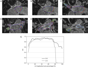
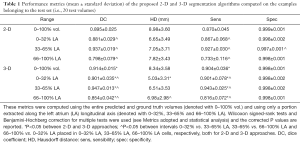
This behavior was further confirmed by the metrics computed in 3 different LA intervals (0–32%, 33–65% and 66–100% LA, see Metrics adopted and statistical analysis) and these results, alongside with the metrics computed for the entire volume (0–100% vol., see Metrics adopted and statistical analysis), are reported in Table 1.

Table 1 Performance metrics (mean ± standard deviation) of the proposed 2-D and 3-D segmentation algorithms computed on the examples belonging to the test set (i.e., 20 test volumes)
Full table

Looking at the DC, the 3-D approach outperformed significantly (P<0.05, see * in Table 1) the 2-D approach in all the tested conditions. In particular, the 3-D and 2-D solutions provided a DC computed in the entire volume of 0.914±0.015 and of 0.895±0.025, respectively. Furthermore, significant differences (P<0.05, see ^ in Table 1) were also found between all the considered ranges of the LA. The same statistical results were obtained for the sensitivity. The HD values were lower in the 3-D pipeline in all the tested conditions but showed significant differences between 2-D and 3-D approaches only for the 0–32% LA (6.65±3.49 and 5.03±3.31 mm, respectively). In addition, in the 3-D pipeline the HD was significantly higher in the 66–100% LA than 0–32% LA.

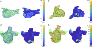
In order to better understand this differential behavior of the performance metrics between LA ranges, we mapped the HD onto the ground truth 3-D meshes and analyzed the maximum distance location within the volume. These visualizations are provided only for the best and worst cases based on the HD values computed on the entire volume (0–100% vol.) and are reported in Figure 4 alongside with the corresponding 3-D segmentation meshes of the predictions and ground truths.

Figure 4 Best (top panels) and worst (bottom panels) cases based on the HD measure as obtained in the 3-D (A,C) and 2-D (B,D) pipelines (3-D best and worst cases: HD=3.37 mm, 17.6 mm; 2-D best and worst cases: HD=3.8 mm, 17.6 mm). In each panel (A-D), the ground truth (green) mesh overlaid with the predicted mesh (blue and red, for the 3-D and 2-D pipelines, respectively) are displayed on the left, while the HD mapped onto the ground truth mesh is displayed on the right.

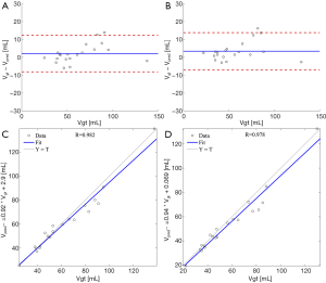
Volumes of the anatomical LA meshes as obtained from the automated analysis were highly correlated with the volumes from ground truth. Bland-Altman analysis between predicted and ground truth volumes showed a bias=2.1 a SD=5.2 mL corresponding to 3.5% and 8.4% respectively, applying the 3-D pipeline (Figure 5A), and a bias=3.5 mL and a SD=5.3 mL corresponding to 5.6% and 8.5% respectively, applying the 2-D pipeline (Figure 5B). In addition, for both 3-D (Figure 5C) and 2-D (Figure 5D) pipelines, linear regression analysis showed excellent correlation coefficients (r=0.982 and r=0.978) and regression lines close to the bisector (3-D: y=0.92x+2.9; 2-D: y=0.94x+0.07).

Figure 5 Results of the Bland-Altman (top panels) and linear regression analysis (bottom panels) on the predicted (V_pred) and ground truth (V_gt) volumes using the 3-D (A,C) and 2-D pipelines (B,D).

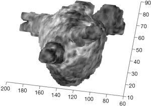
The proposed approach also allows the integration of the LA model with fibrosis information by simply using mean grey-level intensities from LGE MRI in a neighborhood outside the LA cavity surface as a texture of the 3-D anatomical model. An example is reported in Figure 6. This 3-D navigable model allows a qualitative evaluation of the presence of fibrosis and its location.

Figure 6 Example of a representative LA anatomical 3-D model in which mean gray level intensities from LGE MRI in a neighborhood of few voxels outside the LA cavity surface are used as a texture to provide an easy and direct qualitative evaluation of the presence and location of fibrotic tissue. In this specific example, the presence of fibrotic tissue is visible in the inferior wall and on the LA roof. LA, left atrium.

Discussion

The proposed two-stage method produced a joint segmentation of the LA and PVs in AF patients exploiting the Otsu-based localization stage and the fine segmentation stage based on a deep neural network, trained end-to-end from scratch in 2-D and 3-D. Despite the high variability of the LA anatomy, the model provided an accurate prediction that could be useful to support ablation therapy in both the deepened pipelines. Thanks to the fast inference time of this method, the LA surface model was obtained in few seconds (1.01 s for the 3-D pipeline and 0.02 s for the 2-D pipeline, considering only the forward propagation time of a single example through the deep neural network).

The LA segmentations obtained with the proposed 2-D and 3-D approaches showed good and reliable performance, especially for the 3-D pipeline where DC and sensitivity were significantly higher with respect to the 2-D pipeline for all the tested conditions (0–100% vol., 0–32%, 33–65%, 66–100% LA). The same result was obtained by comparing the SDC, that quantifies the disagreement between the predicted and ground truth probability distributions (see Equation 1). Furthermore, the 3-D approach scored always lower HD values than the 2-D approach, with significant lower distances only in the 0–32% LA. The performance improvement observed in the 3-D pipeline might be due to the 3-D convolutional operator exploiting the entire information contained in the 3-D cardiac data. Furthermore, using the 3-D convolution the predicted segmentations were less prone to contain spurious regions and the need of the post-processing step was reduced in the 3-D approach (from 90% to 80% of the predicted segmentations).

In addition, analyzing the best-performing pipeline, DC and sensitivity were significantly lower in the 66–100% LA than in the other two intervals (the same result was obtained by comparing the SDC, see Equation 1), while the HD was only significantly lower in the 66–100% vs. 0–32% LA which was the best predicted interval overall. This phenomenon was further confirmed by looking at the DC computed for each axial slice containing the LA (Figure 3G) and can be further analyzed by mapping the HD onto the ground truth meshes. Indeed, looking to the best and worst cases as reported in Figure 4, higher HD were always found at the PVs. These differences might be due to the high morphological cross-subject variability of the regions near to the mitral valve and the regions containing the PVs. In addition, ground truth meshes included PVs at different depths and consequently no standard rule has been learnt by our CNN-based approach to define to which extent the PVs should be included. This variability in ground truths may also justify such differences.

In the 2-D approach, due to the nature of the convolutional operator introduced in such architecture, the 2-D predictions needed to be stacked together in order to obtain the 3-D predicted segmentation. Conversely, in the 3-D approach the 3-D segmentation was directly computed. Thus, one limit of the 2-D pipeline was the higher number of steps to obtain the final segmentation due to the initial 3-D to 2-D transformation of the input images and the final 2-D to 3-D transformation of the 2-D predictions. In addition, thanks to the 3-D operator exploited in the architecture, in the 3-D pipeline the 3-D predicted surface was smoother and more regular. This difference is particularly clear for the worst segmentations of both the pipelines in Figure 4. Moreover, the 3-D pipeline was characterized by a higher computational cost during the training process: the number of parameters to be optimized increased by 2.91 times (during the first training stage the optimization took up to 320 s/epoch).

The LA mesh volume comparison demonstrated that the 3-D pipeline outperformed the 2-D pipeline. The Bland-Altman comparison showed very small biases; the not negligible limits of agreement were probably due to the not so perfect correspondence between reference and estimated LA contours at the PV level. On note, the PVs should be disconnected before computing the LA volume, a clinical index which has been previously proposed to improve AF patient selection for RFA and correlated to RFA outcome (35). Therefore, the proposed approach may be very useful not only to automatically derive a patient-specific LA anatomical model to support RFA but also to derive LA volume.

Differently from other approaches in which a registration step was required (14,16), in our study a simple mapping of the gray level intensities would make directly available a 3-D model of a target fibrotic tissue distribution on LA surface model obtained from LGE MRI.

In Tao et al. (16), the best results were obtained by comparing the LA chamber model obtained from LGE MRI combined with MRI angiographic data vs. the models from manual tracing; authors reported an average DC equal to 0.86±0.05 in 46 patients. As already highlighted in Introduction, their approach requires substantial computation time due to the extensive computation of the multi-atlas‐based registration.

The proposed workflow represented a good compromise (both in 2-D and 3-D solutions) between performance and number of trainable parameters introduced. Indeed, a 3-D architecture based on V-Net, an architecture adopted in the winning solution of the MICCAI STACOM 2018 Atrial Segmentation Challenge (20), introduces a total number of trainable parameters of 474,362,227 (with 3-D inputs of 80×192×240×1 as in our case, maintaining the same number of feature maps as the U-Net architecture adopted in this study). Thus, our 3-D solution introduced only approx. 1.2% trainable parameters respect to V-Net, representing a more lightweight architecture maintaining competitive performance in the segmentation task. In addition, among the top-5 solutions proposed for the STACOM 2018 challenge, 4 of them (20,36-38) exploited a cascade of two CNNs (one for ROI localization and one for fine segmentation) to solve the segmentation task. Conversely, our two-stage automatic segmentation approach used a first stage ROI localization algorithm that was not data driven (i.e., exploiting Otsu’s algorithm to localize the LA and then crop the input examples). Thus, this methodological choice further reduced the total number of trainable parameters in our approach with respect to (20,36-38). More recently, Xiong et al. (21) reported an overall average DC on 22 LGE MRI data of 0.942. This result was obtained applying a 2-D approach and the performances are higher with respect to our 2-D pipeline tested on 20 LGE MRI data (on average 0.895). However, a similar result was also obtained with our approach with both pipelines (see Table 1) in the central range of LA (33–65% LA). Since in clinical practice PVI is the routine standard ablation procedure, minor accuracy segmentation in this region can be accepted. Conversely, high performance metrics in the central region (3-D: DC=0.947±0.013, HD=6.51±3.53 mm) allow a more robust correspondence between the anatomical model and the presence of fibrosis, thus, this information might be useful for further ablation planning. Notably, despite the dual-path CNN proposed by (19) included 2-D convolutional operators, it introduced 15,448,896 parameters. When dealing with small datasets such the benchmark dataset used in this study, the number of trainable parameters need to be carefully keep limited to avoid overfitting and thus, lightweight deep neural networks may be preferred (with 1,943,761 and 5,647,857 trainable parameters, respectively for ours 2-D and 3-D pipelines). In (21) a direct comparison of AtriaNet with the U-Net was also reported and the average DC for the latter was 0.642. An explanation for this surprisingly low performance compared to our experience using a similar architecture was probably the input data. Indeed, in (21) this metric value was related to a local 41×41 patch of the 2-D axial slice as input and this choice might have affected U-Net performance.

Future developments include the design and development of a new custom loss function and the separation of the PVs structures from the joint segmentation of LA and PVs, evaluating the performance metric solely of the LA chamber without the PVs. In addition, having available the 3-D LA models and patient-specific fibrosis distribution, our approach might be used as the first step for 3-D fibrosis quantification.

Conclusions

In conclusion, we presented a complete two-stage workflow to automatically segment the LA cavity from LGE MRI. Our solution was based on a traditional automatic segmentation algorithm to localize the LA (stage I) and on a 3-D or 2-D CNN to output a fine LA segmentation (stage II). Trained and tested on the MICCAI STACOM 2018 Atrial Segmentation Challenge dataset, the proposed method showed highly accurate LA chamber segmentations compared to the time-consuming manual annotations. In particular, the 3-D pipeline compared to the 2-D pipeline showed significant higher DC and significant lower HD). Furthermore, considering the best-performing pipeline, a differential effect of the performance metrics was found by computing these metrics within different ranges of the LA along the longitudinal axis, with the worst performance in the range containing the PVs. This was associated with higher HD values in correspondence of PVs, which might be due to both the high variability of the PV morphology in the dataset and to a missing consensus for the segmentation of PVs in the ground truth tracings.

Acknowledgments

The authors would like to thank Alessandro Masci and Lorena Esposito for their support in the preliminary conception of the study.

Funding: None.

Footnote

Conflicts of Interest: All authors have completed the ICMJE uniform disclosure form (available at http://dx.doi.org/10.21037/qims-20-168). The authors have no conflicts of interest to declare.

Ethical Statement: The datasets analyzed during the current study are available in the STACOM 2018 Atrial Segmentation Challenge data repository (http://atriaseg2018.cardiacatlas.org/data/). The challenge was organized by the Auckland Bioengineering Institute at the University of Auckland in New Zealand. A large proportion of data were kindly provided by The University of Utah [NIH/NIGMS Center for Integrative Biomedical Computing (CIBC)], while the rest were from multiple other institutes. All clinical data have obtained institutional ethics approval in the Institutions in which they were acquired.

Open Access Statement: This is an Open Access article distributed in accordance with the Creative Commons Attribution-NonCommercial-NoDerivs 4.0 International License (CC BY-NC-ND 4.0), which permits the non-commercial replication and distribution of the article with the strict proviso that no changes or edits are made and the original work is properly cited (including links to both the formal publication through the relevant DOI and the license). See: https://creativecommons.org/licenses/by-nc-nd/4.0/.

References

1. Chugh SS, Blackshear JL, Shen WK, Hamill SC, Gersh BJ. Epidemiology and natural history of atrial fibrillation: clinical implications. J Am Coll Cardiol 2001;37:371-8. [Crossref] [PubMed]
2. Wolf PA, Abbott RD, Kannel WB. Atrial fibrillation as an independent risk factor for stroke: the Framingham study. Stroke 1991;22:983-8. [Crossref] [PubMed]
3. Haïssaguerre M, Jais P, Shah DC, Takahashi A, Hocini M, Quiniou G, Garrigue S, Le Mouroux A, Le Métayer P, Clémenty J. Spontaneous initiation of atrial fibrillation by ectopic beats originating in the pulmonary veins. N Engl J Med 1998;339:659-66. [Crossref] [PubMed]
4. Ouyang F, Tilz R, Chun J, Schmidt B, Wissner E, Zerm T, Neven K, Köktürk B, Konstantinidou M, Metzner A, Fuernkranz A, Kuck KH. Long-term results of catheter ablation in paroxysmal atrial fibrillation clinical perspective: Lessons from a 5-year follow-up. Circulation 2010;122:2368-77. [Crossref] [PubMed]
5. Weerasooriya R, Khairy P, Litalien J, Macle L, Hocini M, Sacher F, Lellouche N, Knecht S, Wright M, Nault I, Miyazaki S, Scavee C, Clementy J, Haissaguerre M, Jais P. Catheter ablation for atrial fibrillation: are results maintained at 5 years of follow-up? J Am Coll Cardiol 2011;57:160-6. [Crossref] [PubMed]
6. Dzeshka MS, Lip GY, Snezhitskiy V, Shantsila E. Cardiac fibrosis in patients with atrial fibrillation: mechanisms and clinical implications. J Am Coll Cardiol 2015;66:943-59. [Crossref] [PubMed]
7. Malcolme-Lawes LC, Juli C, Karim R, Bai W, Quest R, Lim PB, Jamil-Copley S, Kojodjojo P, Ariff B, Davies DW, Rueckert D, Francis DP, Hunter R, Jones D, Boubertakh R, Petersen SE, Schilling R, Kanagaratnam P, Peters NS. Automated analysis of atrial late gadolinium enhancement imaging that correlates with endocardial voltage and clinical outcomes: a 2-center study. Heart Rhythm 2013;10:1184-91. [Crossref] [PubMed]
8. Marrouche NF, Wilber D, Hindricks G, Jais P, Akoum N, Marchlinski F, Kholmovski E, Burgon N, Hu N, Mont L, Deneke T, Duytschaever M, Neumann T, Mansour M, Mahnkopf C, Herweg B, Daoud E, Wissner E, Bansmann P, Brachmann J. Association of atrial tissue fibrosis identified by delayed enhancement MRI and atrial fibrillation catheter ablation: the DECAAF study. JAMA 2014;311:498-506. [Crossref] [PubMed]
9. Zghaib T, Nazarian S. New insights into the use of cardiac magnetic resonance imaging to guide decision-making in AF management. Can J Cardiol 2018;34:1461-70. [Crossref] [PubMed]
10. Giannakidis A, Nyktari E, Keegan J, Pierce I, Horduna IS, Haldar S, Pennell DJ, Mohiaddin R, Wong T, Firmin DN. Rapid automatic segmentation of abnormal tissue in late gadolinium enhancement cardiovascular magnetic resonance images for improved management of long-standing persistent atrial fibrillation. Biomed Eng Online 2015;14:88. [Crossref] [PubMed]
11. Spragg DD, Khurram I, Zimmerman SL, Yarmohammadi H, Barcelon B, Needleman M, Edwards D, Marine JE, Calkins H, Nazarian S. Initial experience with magnetic resonance imaging of atrial scar and co-registration with electroanatomic voltage mapping during atrial fibrillation: success and limitations. Heart Rhythm 2012;9:2003-9. [Crossref] [PubMed]
12. Sohns C, Karim R, Harrison J, Arujuna A, Linton N, Sennett R, Lambert H, Leo G, Williams S, Razavi R, Wright M, Schaeffter T, O'Neill M, Rhode K. Quantitative magnetic resonance imaging analysis of the relationship between contact force and left atrial scar formation after catheter ablation of atrial fibrillation. J Cardiovasc Electrophysiol 2014;25:138-45. [Crossref] [PubMed]
13. Karim R, Housden RJ, Balasubramaniam M, Chen Z, Perry D, Uddin A, Al-Beyatti Y, Palkhi E, Acheampong P, Obom S, Hennemuth A, Lu Y, Bai W, Shi W, Gao Y, Peitgen HO, Radau P, Razavi R, Tannenbaum A, Rueckert D, Cates J, Schaeffter T, Peters D, MacLeod R, Rhode K. Evaluation of current algorithms for segmentation of scar tissue from late gadolinium enhancement cardiovascular magnetic resonance of the left atrium: an open-access grand challenge. J Cardiovasc Magn Reson 2013;15:105. [Crossref] [PubMed]
14. Valinoti M, Fabbri C, Turco D, Mantovan R, Pasini A, Corsi C. 3D patient-specific models for left atrium characterization to support ablation in atrial fibrillation patients. Magnetic Resonance Imaging 2018;45:51-7. [Crossref] [PubMed]
15. Yang G, Zhuang X, Khan H, Haldar S, Nyktari E, Li L, Wage R, Ye X, Slabaugh G, Mohiaddin R, Wong T, Keegan J, Firmin D. Fully automatic segmentation and objective assessment of atrial scars for long-standing persistent atrial fibrillation patients using late gadolinium-enhanced MRI. Medical Physics 2018;45:1562-76. [Crossref] [PubMed]
16. Tao Q, Ipek EG, Shahzad R, Berendsen FF, Nazarian S, van der Geest RJ. Fully automatic segmentation of left atrium and pulmonary veins in late gadolinium-enhanced MRI: towards objective atrial scar assessment. J Magn Reson Imaging 2016;44:346-54. [Crossref] [PubMed]
17. Marciej A. Mazurowski, Buda M, Saha A, Bashir MR. Deep learning in radiology: An overview of the concepts and a survey of the state of the art with focus on MRI. J Magnetic Resonance Imaging 2019;49:939-54. [Crossref]
18. Ghodrati V, Shao J, Bydder M, Zhou Z, Yin W, Nguyen KL, Yang Y, Hu P. MR Image Reconstruction Using Deep Learning: Evaluation of Network Structure and Loss Functions. Quant Imaging Med Surg 2019;9:1516-27. [Crossref] [PubMed]
19. Bian C, Yang X, Ma J, Zheng S, Liu YA, Nezafat R, Heng PA, Zheng Y. Pyramid network with online hard example mining for accurate left atrium segmentation. In: Pop M, Sermesant M, Zhao J, Li S, McLeod K, Young A, Rhode K, Mansi T. (eds.) Statistical Atlases and Computational Models of the Heart. Atrial Segmentation and LV Quantification Challenges. Springer, Cham 2019;237-245.
20. Xia Q, Yao Y, Hu Z, Hao A. Automatic 3d atrial segmentation from lge-mri using volumetric fully convolutional networks. In: Pop M, Sermesant M, Zhao J, Li S, McLeod K, Young A, Rhode K, Mansi T. (eds.) Statistical Atlases and Computational Models of the Heart. Atrial Segmentation and LV Quantification Challenges. Springer, Cham 2019;211-220.
21. Xiong Z, Fedorov V, Fu X, Cheng E, Macleod R, Zhao J. Fully automatic left atrium segmentation from late gadolinium enhanced magnetic resonance imaging using a dual fully convolutional neural network. IEEE Transactions on Medical Imaging 2019;38:515-24. [Crossref] [PubMed]
22. He K, Zhang X, Ren S, Sun J. Delving deep into rectifiers: Surpassing human-level performance on ImageNet classification. In: IEEE International Conference on Computer Vision (ICCV) 2015 arXiv.org/abs/1502.01852
23. Ronneberger O, Fischer P, Brox T. U-net: Convolutional networks for biomedical image segmentation. In: Navab N, Hornegger J, Wells W, Frangi A (eds) Medical Image Computing and Computer-Assisted Intervention – MICCAI 2015. MICCAI 2015. Lecture Notes in Computer Science, vol 9351. Springer, Cham .arXiv.org/abs/1505.04597
24. Ioe S, Szegedy C. Batch normalization: Accelerating deep network training by reducing internal covariate shift. In: 2nd International Conference on Machine Learning 2015;37:448-456, Available online: https://arxiv.org/abs/1502.03167.
25. Srivastava N, Hinton G, Krizhevsky A, Sutskever I, Salakhutdinov R. Dropout: a simple way to prevent neural networks from overfitting. J Mach Learn Res 2014;15:1929-58.
26. Milletari F, Navab N, Ahmadi S. V-net: Fully convolutional neural networks for volumetric medical image segmentation. Computer Vision and Pattern Recognition 2016. Available online: https://arxiv.org/abs/1606.04797
27. Fidon L, Li W, Herrera LCG, Ekanayake J, Kitchen N, Ourselin S, Vercauteren T. Generalised Wasserstein Dice score for imbalanced multi-class segmentation using holistic convolutional networks. Brainlesion: Glioma, Multiple Sclerosis, Stroke and Traumatic Brain Injuries – 3rd International Workshop, BrainLes 2017, held in Conjunction with MICCAI 2017;64-76.
28. Kingma DP, Ba J. Adam: A Method for Stochastic Optimization. In: 3rd International Conference for Learning Representations 2015 arXiv:1412.6980
29. Goodfellow IJ, Warde-Farley D, Mirza M, Courville A, Bengio Y. Maxout networks. In: 30th International Conference on Machine Learning 2013;28:1319-27.
30. Goodfellow I, Bengio Y, Courville A. Deep Learning. MIT Press 2016. Available online: http://www.deeplearningbook.org
31. Chollet F, et al. Keras. GitHub. Available online: https://github.com/fchollet/keras
32. Abadi M, Agarwal A, Barham P, Brevdo E, Chen Z, Citro C, Corrado GS, Davis A, Dean J, Devin M, Ghemawat S, Goodfellow I, Harp A, Irving G, Isard M, Jia Y, Jozefowicz R, Kaiser L, Kudlur M, Levenberg J, Mane D, Monga R, Moore S, Murray D, Olah C, Schuster M, Shlens J, Steiner B, Sutskever I, Talwar K, Tucker P, Vanhoucke V, Vasudevan V, Viegas F, Vinyals O, Warden P, Wattenberg M, Wicke M, Yu Y, Zheng X. TensorFlow: Large-Scale Machine Learning on Heterogeneous Systems (tensorflow.org). Available online: https://arxiv.org/abs/1603.04467
33. Maier-Hein L, Eisenmann M, Reinke A, Onogur S, Stankovic M, Scholz P, Arbel T, Bogunovic H, Bradley AP, Carass A, Feldmann C, Frangi AF, Full PM, van Ginneken B, Hanbury A, Honauer K, Kozubek M, Landman BA, März K, Maier O, Maier-Hein K, Menze BH, Müller H, Neher PF, Niessen W, Rajpoot N, Sharp GC, Sirinukunwattana K, Speidel S, Stock C, Stoyanov D, Taha AA, van der Sommen F, Wang CW, Weber MA, Zheng G, Jannin P, Kopp-Schneider A. Why rankings of biomedical image analysis competitions should be interpreted with care. Nat Commun 2018;9:5217. [Crossref] [PubMed]
34. Benjamini Y, Hochberg Y. Controlling the False Discovery Rate: A Practical and Powerful Approach to Multiple Testing. Journal of the Royal Statistical Society: Series B (Methodological) 1995;57:289-300. [Crossref]
35. Abecasis J, Dourado R, Ferreira A, Saraiva C, Cavaco D, Reis Santos K, Morgado FB, Adragão P, Silva A. Left atrial volume calculated by multidetector computed tomography may predict successful pulmonary vein isolation in catheter ablation of atrial fibrillation. Europace 2009;11:1289-94. [Crossref] [PubMed]
36. Huang N. Available online: 2018.https://www.dropbox.com/s/yyvj4352dax0q26/description_Ning_Huang.pdf?dl=0
37. Yang X, Wang N, Wang Y, Wang X, Nezafat R, Ni D, Heng PA. Combating Uncertainty with Novel Losses for Automatic Left Atrium Segmentation. In: International Workshop on Statistical Atlases and Computational Models of the Heart 2018; 246-254.
38. Liu Y, Dai Y, Yan C, Wang K. Deep Learning Based Method for Left Atrial Segmentation in GE-MRI. In: International Workshop on Statistical Atlases and Computational Models of the Heart 2018; 311-318.