Estimation of changing gross tumor volume from longitudinal CTs during radiation therapy delivery based on a texture analysis with classifier algorithms: a proof-of-concept study

Introduction

Assessing radiation response [change of gross tumor volume (GTV)] during the early stages of radiation therapy (RT) allows the remaining RT to be adapted based on the patient-specific response, enabling the delivery of adaptive RT (ART). CT is by far the most common imaging modality of choice for RT planning and delivery guidance, tumor staging and therapy response monitoring. Using CT imaging to assess response may be subjective and underestimate responses in cases with no apparent changes in tumor size. CT intensity, measured by Hounsfield unit (HU) of attenuation, is stable over time (within 1 HU over the course of treatment), quantitative and sufficiently sensitive to measure small changes (~0.05% change in tissue attenuation coefficient) (1-3). Tumor and surrounding normal tissue may have different physical and biological properties responding differently to therapy; this is reflected in the measured changes in CT texture features. Texture analysis of tumors in CT has revealed tumor heterogeneity and/or treatment responses (4,5).

During image-guided RT (IGRT), noncontrast CT is acquired daily using an in-room CT scanner for patient positioning immediately prior to fraction delivery. It has been shown changes in certain CT histogram features measured from daily CTs are related to the accumulated dose and correlated with treatment outcome for pancreas (1), lung (6), and head and neck (7) cancers. For pancreatic tumors, this variation is small compared with other tumor sites (8-10) and does not differentiate between the tumor region and the rest of the pancreas.

For ART, it is desirable to measure tumor spatial response during RT delivery, e.g., delineating the GTV of the day. A potential method is to use image textures to build an adequate voxel profile, identifying GTV versus adjacent tissue regions within the region of interest (ROI). The aim of this work is to develop such a method estimating the GTV of the day (GTVd) during the course of RT delivery using daily diagnostic-quality CTs acquired with an in-room CT for routine IGRT. Methods of classifying voxels with a varying level of soft tissue and image texture contrasts, lung, breast and pancreas tumors will be used to test and explore different algorithms with the primary goal of detecting the GTV in the lowest contrast case of pancreatic cancer in non-contrast CTs. Classifier algorithms have been used in many fields of study and may be employed to determine regions of similar textures (11-14). Classification is a two-step process that involves first, training on a set of data, and second, evaluating using a separate set of data not included in training (15). The CT dataset closest in time to the diagnostic imaging was used as the baseline to define the voxel-by-voxel labels on the daily CT. The algorithm is validated by comparing location of the tumor region relative to the surrounding tissue in both MRI (GTV as identified by radiology) and daily CT as identified by the classifier.

Methods

Image acquisition

The daily CTs, acquired with 120 kVp with a voxel size of 0.98 mm by 0.98 mm and a slice width of 3 mm using an in-room CT (Definition AS Open, Siemens) during routine IGRT were retrospectively analyzed. The planning MRI was acquired using a 3T MRI scanner (Verio, Siemens); the post-RT/pre-op MRI was obtained on a different 3T scanner (GE Discovery MR750). T1, T2 and ADC images were used for delineation of the pre-RT GTV and post-RT GTV. The contrast-enhanced CT (CCT) was acquired with bolus on a scanner (Discovery CT750, GE). Arterial and hepatic phases were captured with CT using the intensity versus time relationship of the descending aorta.

Contour delineation

The diagnostic GTVs of each site were delineated by the radiologist. GTV was delineated from the planning (pre-RT) images, MRI and/or (CCT) for the breast and pancreas cases, in addition to noncontrast CT for the lung case. This gives the model a ground truth against which the classifier may be trained and tested before it is used for segmenting daily images. The lung is the largest of sites; the sampled lung region is a subset of the planning contour due to shorten computational time during training and testing. In the case of breast, the planning PTV was daily registered and used to define the sampled region. For the pancreas, the PTV included the pancreas head plus a margin. To look at the texture difference only between pancreas and GTV the classifier was restricted to the pancreas head and not the whole PTV.

Feature extraction

To amplify the CT information fed into the classifier, textures were calculated to include the relationship of local variation in the CT intensity. This describes the change in electron density and reflects the material change moving from tissue A to tissue B as the tissue mixture changes within the volume of a voxel and surrounding neighborhood.

The CTs and contours are exported as DICOMs to be read and analyze in Matlab. Textures are calculated for each voxel by taking a 2D neighborhood with a radius of 3, 4 and 5 voxels. Calculated textures include mean, SD, entropy, skewness, kurtosis and Grey Level Co-occurrence Matrix (homogeneity, heterogeneity, correlation and energy) to form the voxel profile further detail is in Table 1 (16). The first order is features based on the average pixel values; the second order is quantifying the relationship between two voxels. These textures quantify features formed by the local variation in CT intensity. To classify spatially dependent changes, a sampling of neighboring voxels around a selected voxel is used to calculate the texture features. This process is repeated for every voxel within the ROI.

Table 1 Summary of the texture used to build the voxel profile. All functions are taken from the Image Processing Toolbox in MATLAB
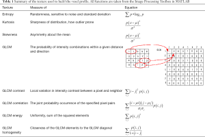
Full table

Model building

We tested a series of classifier algorithms, including the simple tree model, support vector machine (SVM) and k-nearest neighbor algorithm (KNN). The most basic classifier model is a tree model, where the data are split by a series of cuts on the variables. SVM is a logistic regression and is good when the data has exactly two classes. “An SVM classifies data by finding the best hyperplane that separates all data points” (17). KNN is a nonparametric method for classification where the input consists of the k closest training examples in the feature (18). The classification application included in the MATLAB (R2017a) Statistics and Machine Learning Toolbox was used to build and train these classifiers.

The post-RT MRI or CCT is used to delineate the post-RT GTV used to verify the reliability and accuracy of the model’s prediction. The pre/post-RT images are locally registered to the closest in time daily CT images (first or last). Although deformable registration works on many sites, deformable registration with the pancreas was inaccurate due to the blurring effects at the edge of the pancreas. Due to this only local box based rigid registration was used for all cases. Using the blood vessels surrounding the pancreas head to rigidly register the diagnostic imaging to the daily CT was both reliable and re-creatable. Results of registration are used to label the voxel features as GTV or other on the daily CT and are utilized for training a model predicting tissue type on a voxel-by-voxel basis during RT delivery.

Fifty percent of the voxel profiles are reserved for evaluating the model; the remaining 50% are used for training. Texture selection and classifier selection is included together. The classifier is trained initially over multiple classifier algorithms with all textures included to select the best classifier algorithm. Once selected, all combinations of textures are evaluated to maximize the accuracy of the classifier. The trained classifier then is used to process a new daily CT and predict the GTVd, solely based on the trained classifier.

Test patient data

For a given patient, the same CT protocol was used to acquire the daily CTs. Contours of pre-RT GTVs were delineated from the planning images and were populated to the first daily CT based on local registration using MIM (v6.7). Once trained, the classifier is exported and saved to be applied to a new daily CT. A new CT is used to generate new textures and read into the final classifier, to output a label for each voxel forming predicted GTVd. Model-predicted GTVd on the last daily CT was compared with that from the post-RT images (MRI or CCT).

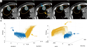
The high-texture contrast case, lung cancer, was treated with 45 Gy in 15 fractions. Because of the high contrast, it was possible to delineate the GTVd using thresholding on a daily CT. No pre- and post-RT images were needed for the lung case. The mean and median CT numbers (CTN) were excluded from the classifier’s list of features as CTN threshold was used in delineating GTV. The patient CT image in Figure 1A shows the GTV contour and the surrounding lung sample used in the feature map calculation and voxel labeling (GTV and LUNG). In Figure 1B, 3D plots of map features give an idea of the cross-feature dependence and the multidimensional separation the classifier is attempting to fit between GTV and surrounding lung.

Figure 1 CT slices of the middle of the identified tumor within the right lung. Series (A) is showing the GTV and the sample lung region used for the classifier. Series (B) shows the multidimensional relationship between the textures. GTV, gross tumor volume.

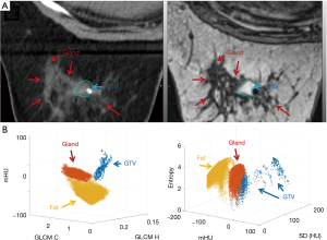
The medium-texture contrast case, breast cancer, was treated with preoperative RT of 30 Gy in 5 fractions followed by lumpectomy. The GTV was generated from the planning MRI and was populated to the first daily CT based on local registration. The GTVs were drawn using the T1, where the tumor is seen as hyperintense/heterogeneous and the normal breast as a spider web of hyper/hypo-intense areas. Figure 2A shows the first daily CT with the GTV; the breast glands of the day were included in the classifier training and Figure 2B shows the texture separation in 3D. Using noncontrast CT, the gland and tumor is not differentiable by eye.

Figure 2 Center slice of the identified tumor within the breast tissue. The T1 on the right is registered to the first daily CT on the left (A). The blue contour is the GTV and the red arrows mark the gland structure. Series (B) shows the multidimensional relationship between the textures (blue is GTV, red is gland, and yellow is fat). GTV, gross tumor volume.

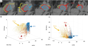
The low-texture contrast cases, pancreatic cancer, was treated with chemotherapy and chemoradiation therapy (CRT) before surgery. The radiation dose was 50.4 Gy in 28 fractions. The pancreatic head was contoured based on the baseline CCT arterial and hepatic phase CTs acquired prior to chemo and post-CRT. This was necessary to avoid including the superior mesenteric vein and superior mesenteric artery within the pancreatic head, which would impact the results due to blood having a slightly higher HU value than the adjacent pancreas. In Figure 3A, the contours of pancreas head and initial (pre-CRT) GTV are shown on the first daily CT. The region between the pre-chemo and pre-CRT GTVs contains fibrosis and is not expected to return structurally to normal pancreas tissue. Figure 3B shows the relationship between textures is dependent on the tissue of interest.

Figure 3 The identified tumor within the pancreas head and texture features. Series (A) is the CT slices of the identified tumor within the pancreas head and series (B) shows the multidimensional relationship between the textures GTV, fibrosis, and normal pancreas tissue. (B) Shows the multidimensional relationship between the textures (blue is GTV, red is fibrosis, and yellow is normal pancreas tissue). GTV, gross tumor volume.

Model evaluation

Dice coefficient (DC) of the model-predicted GTV with the known GTV is used to quantify overlap. The DC is the percent of total overlap between two contours to gauge whether the predicted GTV is within the same region of the ROI. Hausdorff distance (HD) is a measure of how far the edges of the predicted and known GTV are. The HD for two similarly centered contours is a measure of the expansion needed to maximize overlap. For two offset contours, the minimum HD is related to the contour dimension and centroid distance.

Results

Lung tumor texture classification

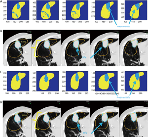
The best fit classifier resulted in an accuracy of 100% using an SVM polynomial. The first day was used for training; eighth and fifteenth days were used for evaluation. The classifier generated map for the eighth day is shown in Figure 4A, along with the daily CT used for texture calculation is shown in Figure 4B. Figure 4C shows the classifier generated map of the last day of RT CT along with the individual CT slices in Figure 4D. The DC for the last day is 84% and eighth day is 83%. In addition, the Hausdorff distance is 1.7 and 1.5 mm for the corresponding days. This is comparable to about 1.5 voxels in the x or y direction or one voxel in the z direction. Table 2 summarizes the final textural combination. In this case, the model settled on a combination of GLCM with standard deviation, entropy, kurtosis, and skewness in all three grid sizes for the textural maps.

Figure 4 The slice by slice comparison of the classifier identified GTV and the seen in CT GTV for lung. Series (A) is generated from the CT taken on the 8th day of RT (B). Series (C) is generated from the CT taken on the 15th day of RT (D). GTV, gross tumor volume.

Table 2 Parameters of the final trained classifiers for lung and breast. The name of the texture is followed by the sample size around a given voxel to calculate the textural maps
Full table

Breast tumor texture classification

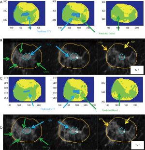
The classifier was trained for regions of fat, gland and GTV. Cross-feature relationships of these regions are shown previously in Figure 2B. The best-fit classifier has an accuracy of 99% for the complex tree and SVM cubic algorithms. The final predictive textures shown in Table 2 are primarily from the same map grid calculated using a 4-voxel radius. The DC for the mid and last day of treatment was 56% and 65%; HDs are 1.4 and 2.2 mm. Figure 5A shows the classifier output on the third treatment compared to the CT slice used to generate the feature map, in Figure 5B. Figure 5C,D show the comparison of the classifier output and the CT for the seventh fraction. The time between the diagnostic image and the first daily CT, to define the test data, is 7 days. After RT the final diagnostic imaging used to delineate the final GTV and register back to the last daily CT was 29 days after the last treatment.

Figure 5 The slice by slice comparison of the Classifier identified GTV and the seen in CT GTV for breast. Series (B) and (D) show the corresponding CT slices versus the trained classifier output in (A) and (C), on the 3rd and 7th treatment respectively. Neither CTs were used in the training. GTV, gross tumor volume.

Pancreas tumor texture classification

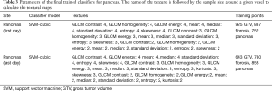
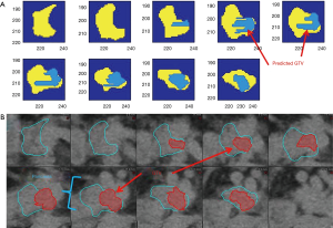
Texture separation in the pancreas case is less pronounced than the previous two sites, the accuracy of the classifier is still high (97% accuracy), as shown previously in Figure 3B by the high degree of overlap in the tissues. The overlap in the textures is seen in the longer list of textures used in the final classifier, which included 24 textures in total (Table 3). Using the first-day CT for training, the DC of the best-case example patient is 61% between the last CT and post-CRT GTV. In addition to the DC, the HD was calculated to be 3.2 mm. Working backwards and using the last daily CT to train the classifier, and then comparing it with the known GTV of the first day, the dice coefficient is 63% with an HD of 2.1 mm. In the context of treatment planning, adding a PTV margin of 3 mm on the GTV may account for the HD. Alternatively, the classifier was run only in the region of pre-chemo and pre-RT GTV with the remaining pancreas expected to be only normal tissue. The DC is 77% for the last treatment compared with the post-CRT diagnostic imaging with an HD of 1.7 mm. Figure 6A is the classifier output and Figure 6B is the corresponding CT contours, where dimensions of a voxel are 0.98 by 0.98 by 3 mm. For resectable and borderline resectable, the initial chemo shrinks the tumor to some degree and the progression of the disease after chemo is within the bounds of the initial GTV. From the pre-RT diagnostic imaging to the first treatment is 5 days and expect little to no detectable change between the two images. Following treatment, the final diagnostic imaging was taken 22 days after the last RT fraction. Due to posttreatment changes, the final GTV is only an estimate of the GTV on the final fraction. The results for all 4 cases are included in Table 4. It is seen that, although the DCs are relatively small due to the small GTVs, the HDs however reflect the classifier defined GTVs are in the regions of the known GTVs when comparing to the GTV dimensions as defined by RECIST.

Table 3 Parameters of the final trained classifiers for pancreas. The name of the texture is followed by the sample size around a given voxel to calculate the textural maps
Full table

Figure 6 The slice by slice comparison of the Classifier identified GTV and the seen in CT GTV for pancreas. (A) is the classifier generated maps generated from the CT slices of the final fraction CT (B). The classifier identifies the potential GTV in blue, yellow is the region identified to be normal or fibrotic tissues. GTV, gross tumor volume.

Table 4 Summary of 4 pancreas cases. The DC and HD calculated between the classifier generated from the textures of the last daily CT and the MR defined projection of the GTV
Full table

Discussion

The learning curve of a classifier depends on classification method, complexity of the classifier and separation of features between distinct groups. In the context of training for a variety of pre-existing conditions with pancreatic cancer (a diabetic pancreas vs. a healthy pancreas vs. a pancreas with intraductal papillary mucinous neoplasm), variance will greatly influence the classifier performance. In addition, pancreatic cancers are characterized by dense fibrous desmoplastic stroma and relatively sparse resulting in an abundance of fibrosis in both the GTV and the treatment response region. Both large and broad ranges of cases are needed to train the classifier, along with cases for model validation. As the complexity and feature overlap increases, so does the need for independent cases. Another aspect of classification is potential bias due to model setup. In this case, contour variation and alignment of planning images to daily CTs could potentially introduce a bias in training and validation sets. Ideally, the training and validation sets would include a variety of cases with multiple versions of contours. The scope of this analysis does not cover more advanced models as deep learning, which requires much larger data sets for training and evaluation due to the variation of the in the treatment response and the pre-treatment state of the pancreas.

For the highest-texture contrast case, lung, a classifier was able to identify the GTV on a consistent basis due to distinct separation in the CT features. For the breast case, classification was sensitive to the separation in CT features between fat to gland, gland to tumor, and fat to tumor, as seen in the 3D plots of features. For pancreas, the lowest-contrast case investigated is a complex organ with a lobular structure; it is almost indistinguishable from surrounding pancreatic tissue on noncontrast CT. Confirmed by pathology, as the tumor volume forms and progresses, the natural structure of the pancreas is altered, and the degree of homogeneity increases. Although the overlap in features is great, this study shows it is possible to identify tumor regions with CT textures. For practical purposes, the classifier should not be patient specific. To do this, the classifier training and evaluation will include the voxel profiles of many patients. The number of patients needed to segment a new patient not used in the training data is dependent on the classification method, complexity of the classifier and how well the groups are separated. For a high-contrast site, such as lung, a simple classifier may be employed on a small cohort of patients with a short list of textures to accurately model the group’s GTV and surrounding lung. As the contrast between regions decreases, more textures are needed to model the different groups. The number of independent datasets (patients) needs to be greater than the number of variates (textures, patient image variation and site-related variation). For the pancreas, the variation in the data is related to noise in CT and differences in the preexisting pancreas. In comparison to lung or breast, many more pancreas cases will be needed to build a complete model.

Utility of a classifier that is trained on a dataset is highly dependent on the quality of the data, in this case, CT images. All of the study sets in this investigation came from the same scanner using the same reconstruction, thus, machine-dependent variation in image quality should be minimal. As previously noted, the time stability of the mean CTN of this scanner has been reported and is on the order of +/− 1 MU over the length of a fractionated therapy plan (1). CT textures are derived from CTN and the machine-related textural stability has also been investigated (2).

Performance of the classifier strongly depends on the site under investigation. Image contrast between the target and surrounding tissue is the highest in lung and the lowest in pancreas, impacting the effectiveness of the classifier to identify the target. Image contrast isn’t the only image quality metric to consider. Breathing motion degrades spatial resolution because in the stationary 3DCT each voxel will contain all tissue types that moved through a voxel at the time of acquisition (19), obscuring the true textures of the target and surrounding tissues. Breathing motion is both location dependent and patient dependent. In comparison to lung and pancreas patients, the breathing-related motion in the breast is negligible.

Image noise (treatment-site and patient specific) is a type of CT texture, which is present in all study sets and will confound classification. Noise in the image is treatment-site and patient specific. No automatic exposure protocol was used to modulate the imaging dose based on the patient width. A larger patient in this study would have more noise in their image due to reduced counting statistics from increased X-ray attenuation. Impact of increased attenuation is also treatment-site specific as an image of a prone breast will benefit from less X-ray attenuation than a pancreas, which is roughly at the center of the abdomen.

A factor that cannot be ruled out in the case of breast and pancreas, the time difference between the dGTV and the final GTV as defined by the diagnostic imaging. As it is a prospective study, the comparison is limited and does not account for the settling from the treatment response. This shows the importance of training on data set with the diagnostic imaging as close in time as possible.

Texture calculated as a map gives the 3D trend in the intensity of an image. Comparing textures is a way to delineate GTV of the day during the course of RT delivery for adaptive RT. Larger studies to develop the utility of using CT texture to quantify and monitor GTV changes in the breast and pancreas are underway. Adaptive planning hinges on the ability to delineate the GTV from the daily RT imaging. Although this is straight forward for high contrast cases, this is a challenge in low contrast regions. By taking the standard daily imaging available and calculating the texture of the regions, it is possible to build a daily GTV model. This is useful in the cases where the GTV is not visible and the organ is expected to go through changes daily.

Acknowledgments

This work is partially supported by the Medical College of Wisconsin Meinerz Foundation and by Siemens Healthineers.

Footnote

Conflicts of Interest: The authors have no conflicts of interest to declare.

References

1. Chen X, Oshima K, Schott D, Wu H, Hall W, Song Y, Tao Y, Li D, Zheng C, Knechtges P, Erickson B, Li XA. Assessment of treatment response during chemoradiation therapy for pancreatic cancer based on quantitative radiomic analysis of daily CTs: An exploratory study. PLoS One 2017;12:e0178961. [Crossref] [PubMed]
2. Plautz TE, Zheng C, Noid G, Li XA. Time stability of delta-radiomics features and the impact on patient analysis in longitudinal CT images. Med Phys 2019;46:1663-76. [Crossref] [PubMed]
3. Watanabe Y. Derivation of linear attenuation coefficients from CT numbers for low-energy photons. Phys Med Biol 1999;44:2201-11. [Crossref] [PubMed]
4. Kiryu S, Akai H, Nojima M, Hasegawa K, Shinkawa H, Kokudo N, Yasaka K, Ohtomo K. Impact of hepatocellular carcinoma heterogeneity on computed tomography as a prognostic indicator. Sci Rep 2017;7:12689. [Crossref] [PubMed]
5. Liu Y, Liu S, Qu F, Li Q, Cheng R, Ye Z. Tumor heterogeneity assessed by texture analysis on contrast-enhanced CT in lung adenocarcinoma: association with pathologic grade. Oncotarget 2017;8:53664-74. [PubMed]
6. Paul J, Yang C, Wu H, Tai A, Dalah E, Zheng C, Johnstone C, Kong FM, Gore E, Li XA. Early Assessment of Treatment Responses During Radiation Therapy for Lung Cancer Using Quantitative Analysis of Daily Computed Tomography. Int J Radiat Oncol Biol Phys 2017;98:463-72. [Crossref] [PubMed]
7. Feng M, Yang C, Chen X, Xu S, Moraru I, Lang J, Schultz C, Li XA. Computed tomography number changes observed during computed tomography-guided radiation therapy for head and neck cancer. Int J Radiat Oncol Biol Phys 2015;91:1041-7. [Crossref] [PubMed]
8. Noid G, Currey AD, Bergom C, Kelly TR, Wadhwa A, Paulson ES, Basir Z, Kong A, Bovi JA, Tai A, Gilat-Schmidt T, Liu Y, Li A. Improvement of Breast Tumor Delineation for Preoperative Radiation Therapy Using Dual-Energy CT. Int J Radiat Oncol Biol Phys 2017;99:E704. [Crossref]
9. Howells CC, Stinauer MA, Diot Q, Westerly DC, Schefter TE, Kavanagh BD, Miften M. Normal liver tissue density dose response in patients treated with stereotactic body radiation therapy for liver metastases. Int J Radiat Oncol Biol Phys 2012;84:e441-6. [Crossref] [PubMed]
10. Danala G, Thai T, Gunderson CC, Moxley KM, Moore K, Mannel RS, Liu H, Zheng B, Qiu Y. Applying Quantitative CT Image Feature Analysis to Predict Response of Ovarian Cancer Patients to Chemotherapy. Acad Radiol 2017;24:1233-9. [Crossref] [PubMed]
11. Robinson ME, O'Shea AM, Craggs JG, Price DD, Letzen JE, Staud R. Comparison of machine classification algorithms for fibromyalgia: neuroimages versus self-report. J Pain 2015;16:472-7. [Crossref] [PubMed]
12. Guyon I, Weston J, Barnhill S, Vapnik V. Gene Selection for Cancer Classification using Support Vector Machines. Mach Learn 2002;46:389-422. [Crossref]
13. Tan K, Li E, Du Q, Du P. An efficient semi-supervised classification approach for hyperspectral imagery. ISPRS J Photogramm Remote Sens 2014;97:36-4. [Crossref]
14. Gillies RJ, Kinahan PE, Hricak H. Radiomics: Images Are More than Pictures, They Are Data. Radiology 2016;278:563-77. [Crossref] [PubMed]
15. Aggarwal CC. Data Classification: Algorithms and Applications 1st ed. Boca Raton, FL: Chapman & Hall/CRC 2014 ISBN 9781466586741.
16. GLCM 2018 “Gray-Level Co-Occurrence Matrix from Image.” Matlab Documentation The Mathworks, Inc. R2018a. Available online: https://www.mathworks.com/help/images/ref/graycomatrix.html
17. SVM 2018 “Support Vector Machines for Binary Classification” Matlab Documentation The Mathworks, Inc. R2018a. Available online: https://www.mathworks.com/help/stats/support-vector-machines-for-binary-classification.html.
18. Coomans D, Massart DL. Alternative k-nearest neighbour rules in supervised pattern recognition: Part 1. k-Nearest neighbour classification by using alternative voting rules. Anal Chim Acta 1982;136:15-27. [Crossref]
19. Yip S, McCall K, Aristophanous M, Chen AB, Aerts HJ, Berbeco R. Comparison of texture features derived from static and respiratory-gated PET images in non-small cell lung cancer. PLoS One 2014;9:e115510. [Crossref] [PubMed]