
A method framework of automatic localization and quantitative segmentation for the cavum septum pellucidum complex and the cerebellar vermis in fetal brain ultrasound images
Introduction
Prenatal care and examination are crucial for gravidas to ensure healthy newborns. Congenital abnormalities of the central nervous system (CNS) are a major concern in prenatal detection of fetal brain (1), which can be screened by ultrasound (US) as a safe, cost-effective, and real-time imaging modality. Evaluation of the corpus callosum (CC) and cerebellar vermis (CV) are critical aspects of fetal brain examination. The CC is a fibrous tract plate connecting the hemispheres, playing a vital role in maintaining coordinated brain activity (2). Congenital malformations like agenesis of the corpus callosum (ACC) and complete agenesis of the corpus callosum (CACC) can lead to mental retardation, epilepsy, and other related symptoms. Similarly, the CV, located in the posterior fossa, plays a vital role in maintaining body equilibrium and coordinating muscle and organ function (3). However, congenital malformations, such as Dandy-Walker malformation (DWM) (4), can lead to the absence, hypoplasia, or rotation of the CV.
During pregnancy, mid-gestational transabdominal scans commonly capture axial plane images of the fetal brain, whereas the mid-sagittal plane offers the most optimal view for visualizing the CC and CV. Three-dimensional (3D) reconstruction technology has improved the display rate of the mid-sagittal plane, allowing physicians to evaluate the CC and CV (2,3). However, artificial evaluation relies on medical expertise and are prone to subjective errors, inefficiencies, and inaccuracies. Thus, there is an urgent need for an accurate and efficient automated method for medical quantification of CC and CV, providing reliable clinical diagnosis.
It is crucial to avoid artificial errors and improve efficiency during examination. However, there is no CC and CV localization and segmentation method that satisfies clinical requirements due to the complexity of FBMUIs for different individuals and the impact of US imaging techniques on image quality. Also, obtaining large-scale datasets is challenging. Therefore, our paper proposes a fully automated method that makes use of the morphological and anatomical characteristics of region of interest (ROI) to explore accurate localization and segmentation, starting from the traditional method, and fulfilling the urgent need for paramedical diagnosis.
The corpus callosum-cavum septum pellucidum complex (CCC) includes the CC and the cavum septum pellucidum (CSP), which are not easily distinguishable in fetal brain mid-sagittal ultrasound images (FBMUIs). Therefore, diagnosis of CC development relies on evaluating the complex. The CSP is a fluid-filled cavity located between two hyaline septa anterior to the brain’s midline, with the CC situated above and the cerebral vault below, and the lateral walls of the hyaline septal lobules (5).
Related works
In recent years, medical image processing techniques have been widely used in assisting medical examinations. Various imaging techniques are used to help physicians make more accurate diagnoses. Traditional and learning-based image analysis methods have been developed for different medical images, lesion areas, and age groups. This paper focuses on 2D US images and proposes a method for accurate localization and segmentation of the CCC and CV. Keywords related to this work include 2D, ultrasound, CCC, CV, localization, and segmentation.
In this paper, we drew inspiration from various studies related to US image analysis, CC, CCC, and CV. These studies included research on the anatomical relationships between these structures (6,7), as well as studies on fetal brain US images (8) and other imaging modalities such as magnetic resonance imaging (MRI) (9-11). We also referenced a processing tool developed for fetal brain MRIs by Rousseau et al. and applied it to the processing of US images (12).
Our research is unique due to the complexity of FBMUIs data and the combination of CCC with CV. However, our approach was inspired by related studies. In this section, we summarize the research related to our paper from the perspectives of CCC and CV, respectively. For the CCC part, the related work mainly focuses on CC.
Related works in CCC
Our paper focused on detecting congenital disorders such as CC and CV hypoplasia in the fetal brain, and we began by reviewing relevant literature from a clinical medical perspective. Previous studies by Pashaj et al. (13) provided a reference range for quantitative characteristics of the fetal CC, and our own previous academic papers established a reference range based on classical medical studies and real clinical experience. With prior anatomical knowledge, we initiated research on CC in fetal brain US images.
To conduct our study, collecting and standardizing experimental data was crucial, with professional anatomical knowledge as the basis. Yang et al. proposed an open benchmark dataset (OpenCC) for CC segmentation and evaluation, created through automatic segmentation and manual refinement methods (14), which could be used to compare and evaluate newly developed CC segmentation algorithms. This dataset also provided ideas for creating FBMUI datasets in our study.
Medical a priori knowledge and a well-developed dataset could assist in localizing and segmenting the CC. Typically, target localization was carried out prior to segmentation in most studies. Due to US image characteristics, our approach used a traditional method to build and analyze the framework. While existing studies primarily used adult brain MRIs, traditional techniques such as the watershed algorithm, active contour model, and level set algorithms were extensively applied for CC localization and segmentation based on image gray value (9). Several traditional methods were used for CC segmentation in brain MRIs, including Freitas et al.’s fully automatic technique using the watershed transform (15), Mogali et al.’s semi-automatic technique using a two-stage snake formulation (16), Li et al.’s fully automatic technique using t1 weighted median and the Geometric Active Contour model (17), and Anandh et al.’s method using anisotropic diffusion filtering and a modified distance regularization level set method for Alzheimer’s brain MRIs (18), which was based on Bayesian inference using sparse representation and multi-atlas voting. Our paper could also benefit from learning-based approaches in terms of data processing methods, among other things. Furthermore, İçer et al. proposed traditional patch-based CC segmentation methods (19-23) as well as denoising and enhancement methods (24) for US images, which encompassed commonly used traditional methods in medical image segmentation. These methods provided valuable references for our research.
Related works in CV
Few studies have focused on CV individuals compared to CC, with most studies instead concentrating on the overall cerebellum structure. Weier et al. provided parametric support for data and quantitative references on cerebellar dysfunction (25), while Joubert et al. analyzed familial CV deficits from medical and genetic perspectives (26). The localization and segmentation of CV rely on prior knowledge of anatomy and well-developed datasets. Our research team has prepared professional medical theory and data support for CV localization and segmentation in FBMUIs (3,27).
Many studies on CV are based on adult brain MRI data and provide references for traditional and learning-based methods. For example, Claude et al. developed a semi-automatic segmentation method for fetal MRI and biometric analysis of posterior fossa midline structures (28), and Hwang et al. proposed an automatic cerebellar extraction method using a shape-guided active contour model in T1-weighted brain MRIs (29). Our paper is more focused on the data processing methods and the rational utilization of medical prior knowledge in learning-based methods, rather than the methods themselves. Powell et al. proposed several automatic segmentation methods using multidimensional registration, including templates, probabilities, artificial neural networks, and support vector machines, and presented a direct comparison of their performance. Their methods may be as reliable as manual scorers and do not require scorer intervention (30).
Our research topic on the localization and segmentation of CCC and CV in FBMUIs is a crucial area in medical image processing, addressing a gap in clinical medical needs. Unlike most studies focusing on MRIs of adult brain, FBMUIs present unique challenges due to the differences in the medium and data processing difficulty. Our paper aims to develop accurate localization and segmentation methods for CCC and CV based on the potential medical and physiological relationship between the two issues.
Methods
The study was conducted in accordance with the Declaration of Helsinki (as revised in 2013). The study was approved by Medical Ethics Committee of Shengjing Hospital, Affiliated to China Medical University (No. 2022PS293K) and informed consent was taken from all the participants.
Overview
The localization and segmentation of the CCC and CV in fetal US images currently rely on manual techniques, which are often inefficient and prone to inaccuracies. In our study, we addressed this clinical challenge by emphasizing two key aspects: target localization and segmentation. Our proposed localization method is based on “Sliding window & Adaptive Average Template”, while the segmentation method is based on “Contour Fitting & Contour Iteration”. The framework’s overall flow is illustrated in Figure 1, leverages the morphological characteristics and spatial location correspondence of the CCC and CV.
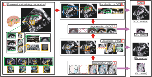
In the first step, we use artificially segmented images as input for a variational autoencoder (VAE) (31,32) for generating average templates of the CCC and CV. An image similarity comparison algorithm applicable to FBMUIs is selected using comparison experiments. In the second and third steps, a progressively more accurate localization structure is applied to the CCC: “Initial Localization-Accurate Localization-Result Detection”. The initial contour is determined using morphological features and segmentation is completed by iterating over the initial contour. In the fourth and fifth steps, the previously obtained CCC segmentation result is used to determine the specific location of the CV. The localization of the CV is completed using the same localization structure as the CCC, based on their physiological geometry relationship. The initial contour determination and subsequent iterative segmentation process are completed based on the localization results of the CV. Figure 2 provides a flowchart illustrating the localization and segmentation process of the CC and CV in FBMUIs. The steps depicted in Figure 2 align precisely with the sequential steps presented in Figure 1.

Framework methodology preparation
Average template images were used for both target localization and segmentation. The localization process was achieved by using image similarity comparison algorithms. The target average template image was generated through training, while the selection of the most suitable image similarity comparison algorithm for US images was based on rigorous comparative experiments.
Data preparation
In our study, fetal brain images were obtained from 140 healthy volunteers with singleton pregnancies, ranging from 20 to 28 weeks of gestational age. US examinations were conducted using GE Voluson E8, GE Voluson E10, and SAMSUNG WS80A machines, equipped with transabdominal 3D transducers (RAB 4-8, RM 6C, or eM6C). Five experienced sonographers, each with more than 10 years of expertise, manually annotated the two-dimensional fetal brain US images in the median sagittal plane of the 3D US data. We only selected images that displayed the complete fetal brain, had no significant sound shadow, and lacked explicit measurement caliper coverage. The original dataset comprised 140 preprocessed images (gray value normalized and size normalized). Two expert sonographers manually annotated the regions corresponding to CCC and CV and provided masks for the two-dimensional fetal brain median sagittal US images. The data collection process adhered to ethical guidelines, and all patients participated with informed consent.
Generation of average templates
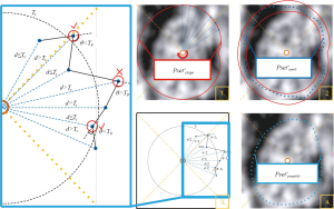
By observing the small image in the upper left corner of Figure 1, the grayscale values of the pixel differences between the main regions of CCC and CV and their background regions in FBMUIs were more significant. This feature reduced human errors in the manual labeling of target images by physicians. The process began with the creation of a training dataset for generating the target average template. A concept called the “pixel domain” was introduced, which represented a line segment of pixel points extending in a specified vector direction with a given length (denoted as a line segment containing n pixel points with width 1 on the image). Taking one side of the CV image A as an example, the micro-adjustment process was illustrated in Figure 3. The main area of the CV, along with its tangent point P1, was identified on the edge E1. A specific length of the pixel domain was determined in the direction of , and a new tangent point was obtained based on the mean pixel value within that range. By applying this method to all four edges, the new target image was obtained. This micro-adjustment process was performed on the 140 FBMUIs manually labeled by doctors to obtain separate CCC and CV image datasets.
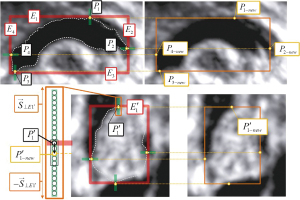
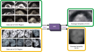
The CCC and CV datasets were divided into three groups following a 5:1:1 ratio (training set: 100, validation set: 20, testing set: 20). These datasets were used as inputs for training the VAE model, which included an encoder and a decoder (22,31). The encoding results of each image were weighted and averaged, and then decoded using the trained decoder. This process yielded the average feature-decoded images for CCC and CV, respectively, which served as the average template images (as shown in Figure 4). These template images contained texture and morphological feature information of the target and background regions. They provided feature comparison information for target localization tasks and an average initial contour for target segmentation tasks, facilitating subsequent segmentation and iteration. Moreover, these template images were combined with the methods described in subsequent chapters to address challenges caused by anatomical variance.
Selection of similarity comparison algorithm
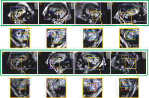
Suitable similarity comparison algorithms were selected through comparative experiments. The average templates of CCC and CV obtained from the original US images served as references for the sliding window search. Algorithms that demonstrated accurate target area localization were then chosen for subsequent localization tasks (as shown in Figure 5). Based on the experimental results, the following algorithms were selected for target localization: Pearson correlation coefficient, structural similarity index measure (SSIM), peak signal-to-noise ratio (PSNR), mutual information (MI), and mean squared error (MSE) (33-36).
Localization of the CCC region
Based on the analysis of 140 clinical images, it was observed that the CCC in FBMUIs generally maintained a consistent orientation with left-right symmetry. However, certain cases exhibited angular deviations. As a result, the localization process for the CCC in FBMUIs comprised the following steps: (step 1) determining the initial search area of CCC; (step 2) performing initial localization using the sliding window search method and a size adaptive template; (step 3) determining the accurate search area based on the initial localization result; (step 4) conducting accurate localization using the sliding window search method and a size adaptive template (different from the initial localization in step 2); (step 5) verifying the accuracy of the localization result and rectifying any potential CCC orientation deviations through rotation if required. Overall, the localization process adhered to a sequential structure known as “Initial Localization-Accurate Localization-Result Detection”.
Initial localization of the CCC region
To determine the initial search region of CCC, we define the concepts of “The Valuable Region” and “The Invaluable Region” (as shown in Figure 6). The area ratio information of these regions is utilized to obtain the fitted rectangular area of the valuable regions (shown as the purple rectangular area in Figure 7), which serves as the initial search area for CCC. A sliding window search is conducted in the initial search area using an average template Tmp1st with an adaptive variable size. The sliding window size matches the template image size. The images obtained from the window are compared with the CCC template image using the correlation coefficient matching algorithm (as shown in Figure 8, step 1). Rectangular boxes of search results that satisfy the similarity threshold range are recorded (as shown in Figure 8, step 2). Subsequently, the centroids of these rectangular boxes are clustered (37), and the centroid of the maximum class is identified as the initial localization result for CCC. The initial localization result of CCC is denoted as Res1st(as shown in Figure 8, step 3).
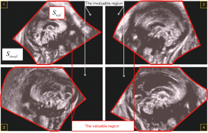
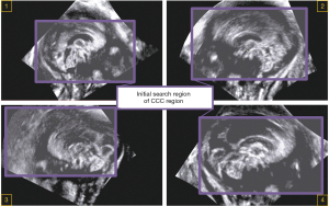
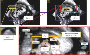
To determine the initial search region of CCC, the concepts of “The Valuable Region” and “The Invaluable Region” were defined (as shown in Figure 6). The area ratio information of these regions was utilized to obtain the fitted rectangular area of the valuable regions (shown as the purple rectangular area in Figure 7), which served as the initial search area for CCC. A sliding window search was conducted in the initial search area using an average template Tmp1st with an adaptive variable size. The sliding window size matched the template image size. The images obtained from the window were compared with the CCC template image using the correlation coefficient matching algorithm (as shown in Figure 8, step 1). Rectangular boxes of search results that satisfied the similarity threshold range were recorded (as shown in Figure 8, step 2). Subsequently, the centroids of these rectangular boxes were clustered (37), and the centroid of the maximum class was identified as the initial localization result for CCC. The initial localization result of CCC was denoted as Res1st (as shown in Figure 8, step 3).
Accurate localization of the CCC region
The accurate search area Rgn2nd was determined based on the initial localization result Res1st (as shown in Figure 9, step 1). By employing the image pyramid and sliding window search, rectangular boxes satisfying the image similarity threshold range (compared with the CCC average template image Tmp2nd) were obtained (as shown in Figure 9, steps 2 and 3). The CCC average template image and similarity comparison algorithms such as SSIM, PSNR, MI, and MSE were utilized for localization (33-36). The top-left point set PTLand bottom-right point set PBR of these rectangular boxes were separately clustered to obtain the geometric centers of the maximum class, denoted as CenTL and CenBR (as shown in Figure 9, step 4). These points were then used as the upper-left corner point and lower-right corner point of the accurate localization results Res2nd (as shown in Figure 9, step 5).
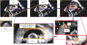
Localization result detection of the CCC region
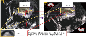
To ensure precise localization that aligned with medical clinical requirements, the mirror symmetry of the morphological features of the CCC was exploited. By comparing the image similarity between the segmented CCC images’ left and right sides, the accuracy of the localization results could be evaluated. Based on the accurate localization result Res2nd, the CCC image Callimg was extracted from the FBMUI. We divided Callimg vertically at its midpoint, obtaining the left and right images CallLeft, CallRight. A mirror inversion operation was performed on CallRight to obtain the image. By applying the normalized correlation coefficient algorithm, the similarity between CallLeft and was compared (as shown in Figure 10). Through extensive experimental comparisons, the threshold value of 0.75 was set for judging the similarity between the left and right images. Upon analyzing the experimental data, we observed that irregular angles in FBMUIs contribute to errors. To mitigate these errors, image rotation was incorporated into the localization method. In the new localization process (as shown in Figure 11), the original CCC localization result was considered as the centroid and its size as the size of the new search area. The original FBMUI was rotated around its center point, with rotation angles ranging from −45° to 45° in 1° increments. Using the same search method employed for accurate CCC localization, CCC was searched within the search area at each angle. This localization process effectively addressed errors arising from variations in shooting angles. The resulting area of the final localization was denoted as Res3rd, and its corresponding CCC image represented the final localization result of CCC, denoted as Callres. By implementing the localization and inspection framework, CCC localization results that met the precision requirements of clinical medicine could be ascertained.

Segmentation of the CCC region
Through medical prior knowledge and careful observations, a significant dissimilarity in grayscale values emerged between the CCC and its surrounding region (as illustrated in Figure 12). Based on this observation, we proposed a pixel comparison-based contour fitting and iterative method for CCC segmentation (18,32,35,38-44).

Contour fitting of the CCC region
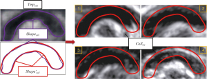
After observation, the shape features of CCC could not be described by conventional geometries. Therefore, the average contour of the average template Tmpcall was adopted to fit the CCC contour and reflect its shape characteristics more accurately (as shown in Figure 13). The purple contour Shapecall represented the average template contour, while the red contour was obtained by smoothing Shapecall.
Contour iteration process of the CCC region
In the CCC images, the outer contour of the fitted map was represented as coordinate points according to the fitting results obtained above, and the fitted contour point set was obtained, denoted as . Due to the differences in the shapes of CCC individuals, the iteration of the CCC contour was completed by adjusting the point set Psetshape (using the pixel information of the main edges of CCC). The specific steps were as follows (as shown in Figure 14).
First, the geometric center point of the image was determined to be Cencall, and N rays were sent out from this point to pass through the points in the point set Psetshape, each in the direction of . For a point Psetshape in the point set Psi, 1≤i≤n, the pixel domain extending along the X direction was found. The coordinates of all points in the pixel domain and the corresponding pixel values were calculated. The coordinates and pixel values of each pixel point in the pixel domain were calculated as follows:
Take a point P(i,m), −10≤m≤10 in Pseti. Suppose this point was , then there was .
In general, the pixel points on the image were discrete (the coordinate values of the pixel points were integer values), and the obtained above could be non-integer values. In such cases, the mean square difference value algorithm was used to obtain the approximate pixel values of coordinate points, denoted as .
By this method, the coordinate information and pixel value information of all the points contained in Pseti were obtained. Then, all the pixel domains of length 5 in the point set Pseti were found, denoted as . The absolute value of the difference between the mean pixel gray value of the first two pixels in each pixel domain was calculated. The mean pixel gray value of the last two pixels was denoted as . The coordinates of the newly obtained point were defined as the coordinates of the maximum absolute value of the difference between the center point Bj of the pixel domain and the above mean value.
All the points in the point set Psetshape were updated by the above process to obtain the new coordinate point set (as shown in Figure 14, steps 1&2). The new point set Psetnew0 was smoothed as follows: in Psetnew0, a neighborhood point set of length N was randomly found (based on the total number of coordinate points contained within the cardinal point set Psetnew0, and experimental comparison, the smoothing effect was best when the length was 7). Assuming that the neighborhood point set was , the average of the horizontal and vertical coordinates of all points in this point set was taken as the new horizontal and vertical coordinate values of the intermediate term in the point set, respectively, and denoted as .
The corresponding coordinate points in the original point set Psetnew0 were replaced by the new coordinate points obtained by the update. Then, a neighboring point clockwise from the updated point set was selected. The newly selected point was used as the center point to determine the new set of coordinate points. The same operation as above was performed to update the coordinates of the center point of the new point set Psetnew0. After finite iterations, the contour points were all updated, and a smooth contour was obtained, which was noted as Psetsoomth0. The contour point set Psetsoomth0 presented on the CCC image was the initial contour of CCC (as shown in Figure 14, steps 3&4).
After obtaining the initial contour of CCC, the initial contour point set of CCC was used as the input point set, and the new contour point set was iterated using the contour point adjustment and smoothing method introduced above. The initial contour point set of CCC was Psetnew0, and the iteration process was as follows:
The contour obtained after a finite number of iterations was the final contour point set of CCC, completing the segmentation of the FBMUI for the subject of CCC.
Localization of the CV region
After the localization and segmentation of the CCC, the subsequent step was to localize the CV (as illustrated in Figure 15). The CV localization process followed the same framework structure as the CCC, adhering to a sequential sequence known as “Initial Localization-Accurate Localization-Result Detection”. However, due to the distinct morphological and spatial characteristics between the CV and CCC, different methods were used within the same framework structure to achieve precise localization of each structure.
Initial localization of the CV region
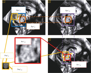
Using medical prior knowledge and anatomical correspondence, the initial search range of CV was derived from the specific location information of CCC. In FBMUIs, there were typically two cases of relative positions between CV and CCC due to the varying positions of the US probe and fetal brain during detection. Thus, the first step involved determining the directionality of CV. With the accurate localization and segmentation results of CCC, two square regions on the left and right were identified as pre-selection search regions for initial CV localization (as shown in Figure 16). After experimental comparison, the square area with a higher mean pixel grayscale value was chosen as the initial localization area of CV, along with its orientation information. Using the same method as initial CCC localization (as shown in Figure 15, step1), the initial localization result of CV in the FBMUI was obtained and denoted as .
Accurate localization of the CV region
The process of accurately localizing the CV region was as follows (refer to Figure 15, steps 2 and 3): To achieve accurate CV localization and obtain reliable localization results, the same methodology utilized for accurate localization of the CCC was adopted. The initial localization result region served as the basis for expansion, allowing the obtainment of the accurate search region for the CV. Subsequently, a sliding window search was performed within this refined search region, and the window images that satisfied the threshold conditions were clustered together. The final accurate localization result of CV was obtained, denoted as .
Localization result detection of the CV region
To ensure localization accuracy in medical clinical settings, the symmetry property of CV in terms of its up-and-down orientation was utilized. The image similarity between the top and bottom sides of the segmented CV images was compared to assess the accuracy of its localization results. From the accurate localization result , the CV image Verimg was extracted from the FBMUI. It was then divided into top and bottom images VerTop, VerBottom by horizontally cutting it in half. A mirror inversion operation was applied to obtain the image. By comparing the similarity between VerBottom and using the normalized correlation coefficient algorithm (as shown in Figure 17), a threshold value of 0.8 was determined based on numerous experimental comparisons. Through this process, CV localization results that satisfied the clinical medical accuracy requirements could be achieved.
Segmentation of the CV region
Through extensive observation and comparison, it became evident that the main part of the CV did not exhibit prominent contrast compared to the surrounding pixels. As illustrated in Figure 18, the outline of the CV appeared blurred. The blue arrows indicated the direction of the CV, while the red arrows served to differentiate the target region from the background. A solid line represented a clear distinction, whereas a dashed line signified an indistinct boundary. Therefore, it became crucial to capitalize on the morphological features of the CV and the interconnection of contour points to achieve its complete segmentation effectively.

Contour fitting of the CV region
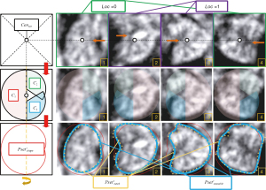
The process of fitting the shape of the CV differed from that of the CCC. Based on prior medical knowledge and extensive observations, the CV shape was simplified as a composite of three fan-shaped surfaces (as depicted in the second row of Figure 19). To determine the CV’s orientation information, the center of the CV image was denoted as Cenver and expanded to conform to the CV shape using the following approach, as illustrated in Figure 19: (I) sector 1 aligned its center coordinates with Cenver; (II) sector 1 had a radius length equal to half the length “L” of the CV image, with a center angle of 180°; (III) sector 2 was positioned 1/8 L above Cenver, with a radius of 3/8 L and a center angle of 120°; (IV) sector 3 was located 1/8 L below Cenver, with a radius of 3/8 L and a center angle of 120°. These sector dimensions were carefully chosen to facilitate obtaining the initial profile of the CV by comparing pixel values from the fit. In our method, the accuracy requirement for the specific shape of the initial fitted contour was not high. Therefore, appropriate radius and angle values were selected to form the fitted profile of the CV. If the orientation coefficient of CV was 0, sector 1 was positioned on the left side of the CV image, while sectors 2 and 3 were on the right side. Conversely, if the orientation coefficient was 1, sector 1 was on the right side, and sectors 2 and 3 were on the left side. Finally, the contour of the combined image of the three sectors served as the initial fitted contour of CV (as shown in the flow on the left side of Figure 19).
Contour iteration process of the CV region
After obtaining the initial fitted contour of CV, it was necessary to iterate over the CV image based on the pixel gray value information to complete the segmentation of CV. After experimental comparison, an iterative method of CV contour based on the comparison of pixel gray values was proposed as follows (as shown in Figure 20):
- First, the central point of the CV image was determined, and a ray was made every 1 degree from the central point. The intersection of these rays with the fitted contour was denoted as
(as shown in Figure 20, step 1).
- The distance between these points and the central point was calculated, denoted as
. Then the average distance between all points in the point set and the central point of the CV image was:
The search interval on each ray was determined as by taking the intersection point as the center point and setting the range to 1/4 Davg of the length. Within each interval, the difference in grayscale values between adjacent pixels was calculated, and the two pixels with the largest difference were identified. The coordinates of the pixel closer to the center of the CV image among these two points were recorded. The pixel points within the search range for each angle were compared and counted, resulting in a new point set denoted as (as shown in Figure 20, step 2). For each point in the newly obtained point set, a judgment was made to identify points that significantly differed from the surrounding points. These points were corrected to achieve smoothing of the point set. The specific operation was as follows (illustrated using point set Pm): to filter out points that were not smooth enough in the newly obtained contour point set, an angle threshold Tθ and a distance threshold Ts corresponding to the point set were proposed. The angle threshold was calculated as the average value of the complementary angles formed by the lines connecting all three adjacent points in the point set.
And the distance threshold was calculated as the average distance between the three points [front , current , and back ] and the center point. After several tests, it was found that this threshold yielded a more desirable distribution of the filtered center point sequence.
For each point in Pm, the two adjacent points before and after it were Pm−1, Pm+1. The angle Pm corresponding to was calculated as the angle between the reverse extension of the ray connecting Pm with its Pm−1 and the line connecting Pm with its Pm−1. And d was the distance from Pm to the center of the CV image. If d was greater than Ts and θ was greater than Tθ, Pm was considered not smooth enough compared to its surrounding points. To smooth the point set, the point on the ray where the non-smooth point was located was determined, and its distance from the center point was replaced with the average of the distances and to the center point (as shown in Figure 20, steps 3&4). All the points in the point set were judged by the above method, and the points that did not meet the requirements were smoothed. Then the smoothed point set was obtained as . To obtain more accurate CV contours, iterative calculations were performed using the above method. was used as a new input for a new round of contour point screening and smoothing, and the iterative process was as follows (as shown in the third row of Figure 19):
Results
Two experiments (Visual Validation and Computational Validation) were conducted to test the accuracy and robustness of our proposed method for target localization, and two additional experiments (Euclidean Distance Validation and Overlapping Percentage Comparison Validation) were conducted to test the effectiveness of the target contour segmentation. The experiments were conducted using real clinical data consisting of 140 US images of the median sagittal plane of the fetal brain. These images were labeled and segmented by experienced physicians to create CCC and CV location and contour information data, which were used as the ground truth (GT). Our method was compared with other comparative methods using various experiments mentioned above to measure the feasibility and accuracy of our method in CCC and CV localization and segmentation tasks. Several measures and statistical tools were used to tabulate the result data for better judgment of the experimental results. The following sections describe the experiments specifically for the localization and segmentation of CCC and CV, respectively.
Validation of the localization of the CCC region
Visual validation
We aimed to verify the feasibility of our proposed framework through both rough and detailed evaluations. In the rough visual verification, we evaluated the framework’s effectiveness in localizing the CCC by comparing the localization results with the GT, i.e., the rectangular area of the CCC marked by physicians. Three evaluation criteria (illustrated in Figure 21) were used to evaluate the results: (I) complete coverage of the CCC region by the localization result box; (II) appropriate size of the localization result box; and (III) correspondence between the center of the CCC region and the center point of the localization result box (with small deviation). The CCC localization results were scored (as shown in Table 1) in terms of “high or low score” and “whether the criterion is satisfied”. “NUM” indicated the number of corresponding scored images in the 140 experimental data, and “PCT” indicated the percentage of the whole data. Based on these observations, statistics, and comparisons, we demonstrated the basic feasibility of our framework for CCC localization.
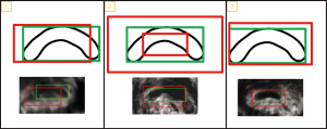
Table 1
| Variables | NUM | PCT (%) |
|---|---|---|
| Score | ||
| 0 | 3/140 | 2.14 |
| 1 | 8/140 | 5.71 |
| 2 | 23/140 | 16.43 |
| 3 | 106/140 | 75.71 |
| Criteria | ||
| ① | 133/140 | 95.00 |
| ② | 127/140 | 90.71 |
| ③ | 121/140 | 86.43 |
CCC, corpus callosum-cavum septum pellucidum complex; NUM, the number of corresponding scored images in the 140 experimental data; PCT, the percentage of the whole data.
Computational validation
An experiment of “computational validation” was conducted to verify the accuracy of CCC localization. The “Intersection over Union (IoU)” values of the CCC localization results and GT were calculated to determine the accuracy (the IoU is defined as (A: the localization result/red box; B: the GT/green box): IoU = (A∪B)/(A∩B). The results are shown in Figure 22, and detailed statistics are presented in Table 2. The method was considered effective when the IoU value was greater than 0.5 based on discussions with front-line clinicians and comparison with results. The overall mean value of IoU was greater than 0.5, indicating the method was effective for CCC localization.
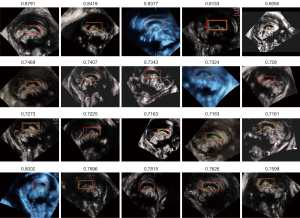
Table 2
| IoU | NUM | PCT (%) | Mean |
|---|---|---|---|
| <0.5 | 11/140 | 7.86 | 0.4040 |
| ≥0.5 | 129/140 | 92.14 | 0.6436 |
| 0.5–0.6 | 43/140 | 30.71 | 0.5605 |
| >0.6–0.7 | 62/140 | 44.29 | 0.6570 |
| >0.7–0.8 | 18/140 | 12.86 | 0.7342 |
| >0.8–0.9 | 6/140 | 4.29 | 0.8304 |
| >0.9 | 0/140 | 0.00 | nan |
IoU: Max =0.8791; Min =0.2936; mean =0.6248. NUM, the number of corresponding scored images in the 140 experimental data; PCT, the percentage of the whole data. IoU, Intersection over Union; CCC, corpus callosum-cavum septum pellucidum complex; nan, not a number.
Validation of the segmentation of the CCC region
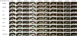
We compared our proposed CCC segmentation method with eight traditional contour segmentation methods, including SNAKE (42), DRLSE (39), C-V (38), RSF (39), ACWE (45), LBF (46), GLFIF (41), and ALF (47), which have been widely used in medical image segmentation. The results of the comparative experiments are shown in Figure 23, which demonstrate the adaptability and accuracy of our method for CCC segmentation.
The Euclidean distance validation
In order to validate the effectiveness CCC segmentation in our proposed framework, we employed a well-established approach for contour comparison: the average minimum Euclidean distance (AMED) between the segmented contour and the corresponding GT (contour labeled by physicians). The results, as presented in Table 3, provide insights into the performance of different segmentation methods. The values in the table represent the mean and standard deviation of AMED, along with the maximum (MAX) and minimum (MIN) values. Our method outperforms other algorithms in terms of data performance, exhibiting the smallest average and extreme values, and demonstrating minimal data fluctuation. This experiment effectively demonstrates the high accuracy and stability of our proposed method.
Table 3
| Methods | Average minimum euclidian distance (px) | ||
|---|---|---|---|
| Mean ± SD | Max | Min | |
| SNAKE | 17.0871±9.6970 | 102.2812 | 6.3644 |
| DRLSE | 19.2121±9.2405 | 99.8596 | 10.6112 |
| C-V | 22.3694±10.4815 | 78.2613 | 5.9222 |
| RSF | 20.3013±9.1172 | 99.4417 | 11.8548 |
| ACWE | 71.4484±18.4213 | 234.9442 | 3.7107 |
| LBF | 11.1675±8.8794 | 88.2111 | 2.8951 |
| GLFIF | 13.5887±9.1329 | 89.7424 | 4.4795 |
| ALF | 14.3849±9.4532 | 69.4153 | 5.4933 |
| Proposed* | 5.0673±3.9653 | 29.1394 | 1.6023 |
*, optimal result. CCC, corpus callosum-cavum septum pellucidum complex; px, pixels; SD, standard deviation; SNAKE, Snakes Active Contour Model; DRLSE, Distance Regularized Level Set Evolution; C-V, Chan-Vese Active Contour Model; RSF, Active Contour Model Based on Region-scalable Fitting; ACWE, Active Contour Without Edges; LBF, Active Contour Model Based on Local Binary Fitting Energy; GLFIF, Global and Local Fuzzy Implicit Active Contours Driven by Weighted Fitting Energy; ALF, Implicit Active Contours Driven by Local Binary Fitting Energy.
Segmentation accuracy comparison validation
The accuracy validation calculation principle is illustrated in Figure 24, where the segmentation accuracy rate RI, missing pixel rate RM and faulting pixel rate RF of the standard profile (red) and the resultant profile (green) are calculated. The statistical information for mean, standard deviation, and MAX values is presented in Table 4. Our segmentation method demonstrated remarkable performance in terms of the mean value and overall stability. There was no significant difference between the MAX value of our method and the comparison method. However, our method consistently achieved the highest MIN value, indicating a more stable performance in CCC segmentation. Furthermore, the mean value of our method for the remaining two rates was the lowest, which demonstrated its exceptional stability and robustness in handling complex and diverse clinical data.

Table 4
| Methods | RI | RM | RF | ||||||||
|---|---|---|---|---|---|---|---|---|---|---|---|
| Mean ± SD | Max | Min | Mean ± SD | Max | Min | Mean ± SD | Max | Min | |||
| SNAKE | 0.8302±0.1159 | 0.9919* | 0.3909 | 0.2866±0.1325 | 0.7184 | 0.0625 | 0.1570±0.1400 | 1.0039* | 0.0056* | ||
| DRLSE | 0.7703±0.1046 | 0.9591 | 0.3645 | 0.2609±0.1282 | 0.7075 | 0.0176 | 0.2318±0.1596 | 1.4651 | 0.0297 | ||
| C-V | 0.8332±0.0982 | 0.9851 | 0.4190 | 0.5136±0.0987 | 0.8216 | 0.2699 | 0.1447±0.1179* | 1.0115 | 0.0093 | ||
| RSF | 0.7423±0.1068 | 0.9440 | 0.3514 | 0.2471±0.1320 | 0.7055 | 0.0150* | 0.2744±0.1731 | 1.5775 | 0.0417 | ||
| ACWE | 0.8580±0.1521 | 0.9854 | 0.4028 | 0.4575±0.1210 | 0.9995 | 0.1466 | 0.1496±0.1925 | 1.9324 | 0.0276 | ||
| LBF | 0.8078±0.1429 | 0.9759 | 0.1959 | 0.3324±0.1490 | 0.7490 | 0.0471 | 0.1641±0.1398 | 1.0173 | 0.0168 | ||
| GLFIF | 0.8262±0.1139 | 0.9997 | 0.3428 | 0.4197±0.1367 | 0.9894 | 0.1105 | 0.1577±0.1302 | 1.2228 | 0.0340 | ||
| ALF | 0.7931±0.1116 | 0.9644 | 0.2045 | 0.2724±0.1354 | 0.8688 | 0.0314 | 0.1973±0.1409 | 1.2269 | 0.0245 | ||
| Proposed | 0.8740*±0.0883* | 0.9680 | 0.4281* | 0.1508*±0.0913* | 0.5760* | 0.0188 | 0.1406*±0.1560 | 1.2588 | 0.0201 | ||
*, optimal result. CCC, corpus callosum-cavum septum pellucidum complex; RI, segmentation accuracy rate; RM, missing pixel rate; RF, faulting pixel rate; SD, standard deviation; SNAKE, Snakes Active Contour Model; DRLSE, Distance Regularized Level Set Evolution; C-V, Chan-Vese Active Contour Model; RSF, Active Contour Model Based on Region-scalable Fitting; ACWE, Active Contour Without Edges; LBF, Active Contour Model Based on Local Binary Fitting Energy; GLFIF, Global and Local Fuzzy Implicit Active Contours Driven by Weighted Fitting Energy; ALF, Implicit Active Contours Driven by Local Binary Fitting Energy.
Segmentation results mask image similarity comparison validation
The performance of our CCC segmentation method was evaluated by comparing the similarity between the segmentation result and the GT mask images using five standard parameters: Kendall rank correlation (KRC), dice similarity coefficient (DSC), SSIM, Hausdorff distance (HD), and average Hausdorff distance (AHD) (46,48). The results, presented in Table 5, clearly indicated that our method outperformed other approaches across multiple parameters (higher mean values and lower standard deviations). Moreover, the DSC results of 30 CCC images, presented in Table 6, further validated our method’s superiority over alternative techniques. These statistical analyses validated the accuracy, robustness, and stability of our method for CCC segmentation.
Table 5
| Methods | KRC, mean ± SD | DSC, mean ± SD | SSIM, mean ± SD | HD, mean ± SD (px) | AHD, mean ± SD (px) |
|---|---|---|---|---|---|
| SNAKE | 0.6735±0.1157 | 0.7603±0.0879 | 0.7636±0.0529 | 55.3089±26.8671 | 3.5231±4.6711 |
| DRLSE | 0.6444±0.0982 | 0.7236±0.0753 | 0.7447±0.0412 | 54.6655±25.8281 | 3.8592±4.3156 |
| C-V | 0.5968±0.1033 | 0.7943±0.0839 | 0.6836±0.0677 | 75.1000±29.8133 | 3.8606±5.0408 |
| RSF | 0.6338±0.0966 | 0.7061±0.0741 | 0.7393±0.0410* | 56.3961±25.4791 | 4.1356±4.2407 |
| ACWE | 0.6513±0.1739 | 0.8223±0.1209 | 0.7319±0.0926 | 56.0623±27.2610 | 2.8226±5.6080 |
| LBF | 0.6204±0.1907 | 0.7624±0.1176 | 0.7005±0.1202 | 66.7879±38.9074 | 3.8926±5.2375 |
| GLFIF | 0.6396±0.1517 | 0.7956±0.1013 | 0.6952±0.0930 | 79.9539±34.5955 | 3.7200±4.7642 |
| ALF | 0.6296±0.1455 | 0.6050±0.0857 | 0.6693±0.0685 | 106.8502±24.2695 | 9.2019±3.9525 |
| Proposed | 0.8312*±0.0669* | 0.8955*±0.0483* | 0.8475*±0.0499 | 28.4420*±20.2059* | 0.7071*±1.2097* |
*, optimal result. CCC, corpus callosum-cavum septum pellucidum complex; KRC, Kendall rank correlation; DSC, dice similarity coefficient; SSIM, structural similarity index measure; HD, Hausdorff distance; AHD, average Hausdorff distance; SD, standard deviation; px, pixels; SNAKE, Snakes Active Contour Model; DRLSE, Distance Regularized Level Set Evolution; C-V, Chan-Vese Active Contour Model; RSF, Active Contour Model Based on Region-scalable Fitting; ACWE, Active Contour Without Edges; LBF, Active Contour Model Based on Local Binary Fitting Energy; GLFIF, Global and Local Fuzzy Implicit Active Contours Driven by Weighted Fitting Energy; ALF, Implicit Active Contours Driven by Local Binary Fitting Energy.
Table 6
| Exp. | DSC | ||||||||
|---|---|---|---|---|---|---|---|---|---|
| SNAKE | DRLSE | C-V | RSF | ACWE | LBF | GLFIF | ALF | Proposed | |
| 1 | 0.8561 | 0.7933 | 0.8520 | 0.7783 | 0.8638 | 0.7970 | 0.8428 | 0.6206 | 0.9333* |
| 2 | 0.7936 | 0.7368 | 0.7735 | 0.7234 | 0.8009 | 0.7480 | 0.7321 | 0.5366 | 0.9215* |
| 3 | 0.8527 | 0.8137 | 0.7713 | 0.8001 | 0.7719 | 0.8011 | 0.7402 | 0.5719 | 0.9267* |
| 4 | 0.7525 | 0.7197 | 0.8694 | 0.7043 | 0.9027* | 0.5171 | 0.7661 | 0.5448 | 0.9014 |
| 5 | 0.8437 | 0.7538 | 0.8443 | 0.7333 | 0.8665 | 0.8560 | 0.8541 | 0.6000 | 0.9090* |
| 6 | 0.7400 | 0.7511 | 0.8142 | 0.7359 | 0.8148 | 0.7883 | 0.8150 | 0.5738 | 0.8818* |
| 7 | 0.7494 | 0.8041 | 0.8521 | 0.7822 | 0.8679 | 0.8369 | 0.8807 | 0.6639 | 0.8933* |
| 8 | 0.8245 | 0.8142 | 0.8296 | 0.7861 | 0.8339 | 0.8766 | 0.8619 | 0.6733 | 0.9179* |
| 9 | 0.7573 | 0.6455 | 0.8040 | 0.6250 | 0.8072 | 0.8020 | 0.8374 | 0.6023 | 0.9058* |
| 10 | 0.7071 | 0.7050 | 0.8452 | 0.6807 | 0.8587 | 0.7862 | 0.8094 | 0.7394 | 0.8695* |
| 11 | 0.7998 | 0.7870 | 0.8882 | 0.7705 | 0.8923 | 0.7764 | 0.9078 | 0.6446 | 0.9336* |
| 12 | 0.8275 | 0.7836 | 0.8965 | 0.7622 | 0.9082 | 0.8147 | 0.8969 | 0.6730 | 0.9147* |
| 13 | 0.8470 | 0.7977 | 0.8809 | 0.7789 | 0.8847 | 0.8860 | 0.8651 | 0.6686 | 0.9341* |
| 14 | 0.8107 | 0.7990 | 0.8612 | 0.7809 | 0.8523 | 0.8463 | 0.8601 | 0.6664 | 0.9138* |
| 15 | 0.7855 | 0.7662 | 0.7921 | 0.7502 | 0.8666 | 0.7853 | 0.7810 | 0.6213 | 0.9290* |
| 16 | 0.7774 | 0.6941 | 0.8514 | 0.6769 | 0.8766 | 0.7613 | 0.8600 | 0.5617 | 0.9313* |
| 17 | 0.7802 | 0.7022 | 0.8081 | 0.6856 | 0.8636 | 0.7677 | 0.8406 | 0.5470 | 0.9182* |
| 18 | 0.7745 | 0.7762 | 0.8423 | 0.7652 | 0.8594 | 0.7314 | 0.8199 | 0.5816 | 0.9187* |
| 19 | 0.6188 | 0.5556 | 0.7986 | 0.5414 | 0.8033 | 0.5457 | 0.7675 | 0.4806 | 0.9080* |
| 20 | 0.6667 | 0.6330 | 0.7022 | 0.6312 | 0.8231 | 0.6949 | 0.6842 | 0.5481 | 0.9327* |
| 21 | 0.7639 | 0.7126 | 0.7757 | 0.7010 | 0.8173 | 0.7651 | 0.8202 | 0.5452 | 0.9052* |
| 22 | 0.8450 | 0.8002 | 0.8236 | 0.7772 | 0.8668 | 0.8558 | 0.8467 | 0.6338 | 0.9225* |
| 23 | 0.8490 | 0.7378 | 0.8310 | 0.7219 | 0.8711 | 0.8209 | 0.8229 | 0.6293 | 0.9192* |
| 24 | 0.7493 | 0.6242 | 0.7103 | 0.6026 | 0.7283 | 0.7490 | 0.7066 | 0.5578 | 0.8766* |
| 25 | 0.8614 | 0.7952 | 0.8010 | 0.7779 | 0.8256 | 0.8469 | 0.8729 | 0.5680 | 0.8900* |
| 26 | 0.7907 | 0.7137 | 0.6774 | 0.7129 | 0.7556 | 0.7658 | 0.6671 | 0.4771 | 0.8068* |
| 27 | 0.4026 | 0.5794 | 0.6406 | 0.5523 | 0.6377 | 0.5897 | 0.6399 | 0.4377 | 0.8353* |
| 28 | 0.8143 | 0.7282 | 0.9074* | 0.7042 | 0.8901 | 0.8124 | 0.8746 | 0.7208 | 0.7530 |
| 29 | 0.6849 | 0.6190 | 0.6389 | 0.6001 | 0.6594 | 0.6872 | 0.6353 | 0.4807 | 0.8432* |
| 30 | 0.8603 | 0.7999 | 0.8304 | 0.7874 | 0.8573 | 0.8272 | 0.8584 | 0.5796 | 0.9029* |
*, optimal result. CCC, corpus callosum-cavum septum pellucidum complex; Exp., experiment; DSC, dice similarity coefficient; SNAKE, Snakes Active Contour Model; DRLSE, Distance Regularized Level Set Evolution; C-V, Chan-Vese Active Contour Model; RSF, Active Contour Model Based on Region-scalable Fitting; ACWE, Active Contour Without Edges; LBF, Active Contour Model Based on Local Binary Fitting Energy; GLFIF, Global and Local Fuzzy Implicit Active Contours Driven by Weighted Fitting Energy; ALF, Implicit Active Contours Driven by Local Binary Fitting Energy.
Validation of the localization of the CV region
Visual validation
The evaluation of CV localization and segmentation methods was conducted using the same criteria as CCC, and the results were presented in Table 7. Among the 141 images examined, an impressive 105 images achieved a localization score of 3, accounting for nearly 75% of the total results. In terms of segmentation, a significant majority of images met criterion 2, accounting for nearly 94% of the cases. The localization results for CV demonstrated a superior performance in criterion 2 compared to the localization results for CCC. This suggested that our CV localization method was more sensitive to size variations and demonstrated remarkable adaptability in addressing the substantial disparities observed in clinical images.
Table 7
| Variables | NUM | PCT (%) |
|---|---|---|
| Score | ||
| 0 | 4/140 | 2.86 |
| 1 | 5/140 | 3.57 |
| 2 | 26/140 | 18.57 |
| 3 | 105/140 | 75.00 |
| Criteria | ||
| ① | 122/140 | 87.14 |
| ② | 131/140 | 93.57 |
| ③ | 119/140 | 85.00 |
CV, cerebellar vermis; NUM, the number of corresponding scored images in the 140 experimental data; PCT, the percentage of the whole data.
Computational validation
The localization results of CV were presented in Figure 25 and summarized in Table 8. The majority of IoU values ranged between 0.6 and 0.7, with 87.14% of the results satisfying the accuracy requirement. It is important to note that this accuracy level was slightly lower than that of CCC localization, where 92.14% of the results met the accuracy requirement. This slight decrease in accuracy could be attributed to the integrated serial structure of our method. The localization and segmentation outcomes of CCC could have an impact on the subsequent localization and segmentation process of CV. Nevertheless, our method still provided relatively good results for the localization of CV.
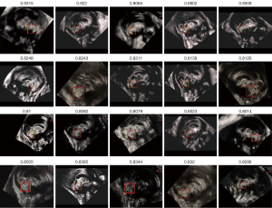
Table 8
| IoU | NUM | PCT (%) | Mean |
|---|---|---|---|
| <0.5 | 18/140 | 12.86 | 0.4535 |
| ≥0.5 | 122/140 | 87.14 | 0.6846 |
| 0.5–0.6 | 29/140 | 20.71 | 0.5548 |
| >0.6–0.7 | 39/140 | 27.86 | 0.6479 |
| >0.7–0.8 | 34/140 | 24.29 | 0.7451 |
| >0.8–0.9 | 17/140 | 12.14 | 0.8265 |
| >0.9 | 3/140 | 2.14 | 0.9200 |
IoU: Max =0.9315; Min =0.4255; mean =0.6548. IoU, Intersection over Union; CV, cerebellar vermis; NUM, the number of corresponding scored images in the 140 experimental data; PCT, the percentage of the whole data.
Validation of the segmentation of the CV region
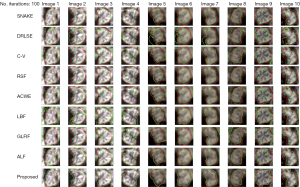
In this section, the experimental methods, the criteria for judging the results, and the way the tables were documented were identical to those in section “Validation of the segmentation of the CCC region”. The description of the experimental principle was omitted. The experimental results were shown in Figure 26.
The Euclidean distance validation
Table 9 illustrated the outstanding performance of our method in terms of the mean and AMED value when compared to the other 8 algorithms (highlighted by asterisks). Our method exhibited a significant advantage in achieving the optimal mean value. Furthermore, the standard deviation of the mean value for our method was the smallest among the compared algorithms, indicating its exceptional stability. Hence, it could be concluded that our framework’s CV segmentation contour accurately and effectively represented the true contour of CV in FBMUIs.
Table 9
| Methods | Average minimum euclidian distance (px) | ||
|---|---|---|---|
| Mean ± SD | Max | Min | |
| SNAKE | 26.2120±6.7847 | 52.1724 | 7.9756 |
| DRLSE | 20.5157±5.6312 | 37.3987 | 8.7888 |
| C-V | 17.8330±4.8314 | 35.0913 | 7.6370 |
| RSF | 33.6351±7.9459 | 57.7634 | 15.6956 |
| ACWE | 34.7071±8.6887 | 101.6779 | 11.8902 |
| LBF | 12.2416±4.3219 | 29.8167 | 4.5964 |
| GLFIF | 20.0284±9.0308 | 65.1474 | 5.8798 |
| ALF | 17.0995±9.5254 | 54.1683 | 5.7958 |
| Proposed* | 6.9800±3.6554 | 24.1876 | 2.1183 |
*, optimal result. CV, cerebellar vermis; px, pixels; SD, standard deviation; SNAKE, Snakes Active Contour Model; DRLSE, Distance Regularized Level Set Evolution; C-V, Chan-Vese Active Contour Model; RSF, Active Contour Model Based on Region-scalable Fitting; ACWE, Active Contour Without Edges; LBF, Active Contour Model Based on Local Binary Fitting Energy; GLFIF, Global and Local Fuzzy Implicit Active Contours Driven by Weighted Fitting Energy; ALF, Implicit Active Contours Driven by Local Binary Fitting Energy.
Segmentation accuracy comparison validation
The experimental principle was the same as that shown in Figure 24, and the corresponding statistical results were presented in Table 10. The SNAKE and RSF segmentation methods yielded a MIN value of 0.0000 for the missing pixel rate because their contours completely contained the manual marker contours. However, to ensure contour smoothness and integrity, the fitting degree between the contour result and the true edge of the target was sacrificed, leading to inaccurate results. Given the complexity of the CV contour, our method improved contour accuracy by smoothing and iterating within a small range.
Table 10
| Methods | RI | RM | RF | ||||||||
|---|---|---|---|---|---|---|---|---|---|---|---|
| Mean ± SD | Max | Min | Mean ± SD | Max | Min | Mean ± SD | Max | Min | |||
| SNAKE | 0.8067±0.0899 | 0.9955 | 0.5647 | 0.0923±0.0820 | 0.3781 | 0.0000* | 0.2380±0.1435 | 0.6728 | 0.0032 | ||
| DRLSE | 0.8033±0.0755 | 0.9483 | 0.5809 | 0.3305±0.1011 | 0.6211 | 0.0708 | 0.1785±0.1052 | 0.6348 | 0.0238 | ||
| C-V | 0.9032±0.0623 | 0.9978* | 0.7158 | 0.3403±0.1119 | 0.5969 | 0.0409 | 0.1672±0.0524* | 0.4178 | 0.0009* | ||
| RSF | 0.7238±0.0904 | 0.9743 | 0.5062 | 0.0613*±0.0680* | 0.3132* | 0.0000* | 0.3841±0.1780 | 0.9627 | 0.0218 | ||
| ACWE | 0.6692±0.2466 | 0.9964 | 0.0199 | 0.3317±0.1734 | 0.9753 | 0.0000* | 0.5663±0.7907 | 4.7464 | 0.0021 | ||
| LBF | 0.6951±0.1473* | 0.9621 | 0.3326 | 0.1901±0.1209 | 0.5399 | 0.0047 | 0.3969±0.2667 | 1.2833 | 0.0318 | ||
| GLFIF | 0.7871±0.1492 | 0.9946 | 0.2443 | 0.3728±0.1275 | 0.8286 | 0.0450 | 0.1909±0.1632 | 0.8888 | 0.0030 | ||
| ALF | 0.8203±0.0805 | 0.9948 | 0.5542 | 0.1055±0.0813 | 0.3543 | 0.0015 | 0.2118±0.1249 | 0.6938 | 0.0037 | ||
| Proposed | 0.9114±0.0576 | 0.9842 | 0.7223* | 0.1268±0.0713 | 0.3812 | 0.0192 | 0.0904±0.0693 | 0.3668* | 0.0121 | ||
*, optimal result. CV, cerebellar vermis; RI, segmentation accuracy rate; RM, missing pixel rate; RF, faulting pixel rate; SD, standard deviation; SNAKE, Snakes Active Contour Model; DRLSE, Distance Regularized Level Set Evolution; C-V, Chan-Vese Active Contour Model; RSF, Active Contour Model Based on Region-scalable Fitting; ACWE, Active Contour Without Edges; LBF, Active Contour Model Based on Local Binary Fitting Energy; GLFIF, Global and Local Fuzzy Implicit Active Contours Driven by Weighted Fitting Energy; ALF, Implicit Active Contours Driven by Local Binary Fitting Energy.
Segmentation results mask image similarity comparison validation
In “Segmentation accuracy comparison validation” under section “Validation of the segmentation of the CCC region”, five standard parameters were chosen to calculate the mask image similarity. The same parameters were used in this section and the results are shown in Tables 11,12. Our method achieved better results in most cases (highlighted by asterisks in the tables), indicating its accuracy, robustness, and stability for CV segmentation.
Table 11
| Methods | KRC, mean ± SD | DSC, mean ± SD | SSIM, mean ± SD | HD, mean ± SD (px) | AHD, mean ± SD (px) |
|---|---|---|---|---|---|
| SNAKE | 0.7092±0.0689 | 0.7657±0.0518 | 0.7197±0.0617 | 43.4975±9.1751 | 2.3571±0.9083 |
| DRLSE | 0.4766±0.1032 | 0.7479±0.0394 | 0.5883±0.0577 | 40.5972±8.0527* | 2.4787±0.7693 |
| C-V | 0.5430±0.1276 | 0.7919±0.0530 | 0.6652±0.0711 | 44.7217±10.8316 | 2.2609±1.0468 |
| RSF | 0.6552±0.0650 | 0.7014±0.0489 | 0.6715±0.0659 | 47.4939±8.6269 | 3.3596±1.0448 |
| ACWE | 0.3882±0.2172 | 0.6391±0.1731 | 0.5636±0.1181 | 61.1534±24.1471 | 6.1888±5.7705 |
| LBF | 0.5928±0.1676 | 0.7883±0.0568 | 0.6030±0.1424 | 37.9273±10.8149 | 1.4088±0.6966 |
| GLFIF | 0.4232±0.1621 | 0.7547±0.0687 | 0.5715±0.1023 | 50.8752±9.2979 | 2.6910±1.1194 |
| ALF | 0.7026±0.0688 | 0.7332±0.0525 | 0.6794±0.0540 | 58.2279±9.1697 | 3.1669±1.0745 |
| Proposed | 0.8154*±0.0603* | 0.9116*±0.0309* | 0.8144*±0.0454* | 22.6455*±8.7203 | 0.4377*±0.3673* |
*, optimal result. CV, cerebellar vermis; KRC, Kendall Rank Correlation; DSC, Dice Similarity Coefficient; SSIM, Structural Similarity Index Measure; HD, Hausdorff Distance; AHD, Average Hausdorff Distance; SD, standard deviation; px, pixels; SNAKE, Snakes Active Contour Model; DRLSE, Distance Regularized Level Set Evolution; C-V, Chan-Vese Active Contour Model; RSF, Active Contour Model Based on Region-scalable Fitting; ACWE, Active Contour Without Edges; LBF, Active Contour Model Based on Local Binary Fitting Energy; GLFIF, Global and Local Fuzzy Implicit Active Contours Driven by Weighted Fitting Energy; ALF, Implicit Active Contours Driven by Local Binary Fitting Energy.
Table 12
| Exp. | DSC | ||||||||
|---|---|---|---|---|---|---|---|---|---|
| SNAKE | DRLSE | C-V | RSF | ACWE | LBF | GLFIF | ALF | Proposed* | |
| 1 | 0.8176 | 0.7237 | 0.7377 | 0.7372 | 0.7741 | 0.6224 | 0.7423 | 0.6897 | 0.9370 |
| 2 | 0.7348 | 0.6872 | 0.8104 | 0.6552 | 0.7177 | 0.7172 | 0.8212 | 0.7965 | 0.9443 |
| 3 | 0.8352 | 0.7400 | 0.7856 | 0.7492 | 0.7547 | 0.6986 | 0.7791 | 0.7468 | 0.9494 |
| 4 | 0.7887 | 0.6540 | 0.8376 | 0.6682 | 0.3159 | 0.7046 | 0.8322 | 0.7984 | 0.9578 |
| 5 | 0.7407 | 0.6979 | 0.7385 | 0.7476 | 0.7219 | 0.8523 | 0.7489 | 0.6558 | 0.9288 |
| 6 | 0.8028 | 0.6962 | 0.8005 | 0.7553 | 0.7864 | 0.8956 | 0.8118 | 0.7221 | 0.9508 |
| 7 | 0.7825 | 0.7060 | 0.8879 | 0.7204 | 0.8326 | 0.8609 | 0.8612 | 0.7304 | 0.9212 |
| 8 | 0.8342 | 0.7700 | 0.7956 | 0.8094 | 0.7620 | 0.9001 | 0.7524 | 0.6293 | 0.9047 |
| 9 | 0.7397 | 0.7415 | 0.8800 | 0.6236 | 0.5726 | 0.7644 | 0.8481 | 0.8229 | 0.9365 |
| 10 | 0.7185 | 0.6735 | 0.7625 | 0.6735 | 0.6532 | 0.7382 | 0.7164 | 0.7396 | 0.8553 |
| 11 | 0.7478 | 0.7508 | 0.7579 | 0.7343 | 0.4239 | 0.7014 | 0.6656 | 0.6891 | 0.9084 |
| 12 | 0.6341 | 0.6538 | 0.8370 | 0.5872 | 0.4910 | 0.7668 | 0.7522 | 0.7765 | 0.8541 |
| 13 | 0.7058 | 0.7161 | 0.7830 | 0.6302 | 0.4799 | 0.6937 | 0.7576 | 0.8365 | 0.9174 |
| 14 | 0.8172 | 0.7352 | 0.7078 | 0.7689 | 0.6925 | 0.7410 | 0.6991 | 0.6750 | 0.9518 |
| 15 | 0.8161 | 0.6970 | 0.8370 | 0.7128 | 0.8047 | 0.7935 | 0.8275 | 0.7840 | 0.9219 |
| 16 | 0.7563 | 0.7545 | 0.8476 | 0.7002 | 0.8193 | 0.8096 | 0.8159 | 0.7490 | 0.9562 |
| 17 | 0.7725 | 0.6490 | 0.8406 | 0.7310 | 0.7836 | 0.8185 | 0.8039 | 0.6652 | 0.9246 |
| 18 | 0.7748 | 0.6974 | 0.6767 | 0.7495 | 0.6163 | 0.7241 | 0.6665 | 0.6905 | 0.9386 |
| 19 | 0.7818 | 0.7239 | 0.7501 | 0.6876 | 0.6990 | 0.7764 | 0.7483 | 0.7793 | 0.9383 |
| 20 | 0.7352 | 0.6879 | 0.7803 | 0.6562 | 0.6413 | 0.7916 | 0.8153 | 0.7488 | 0.9036 |
| 21 | 0.7813 | 0.7730 | 0.7670 | 0.7145 | 0.6188 | 0.8438 | 0.7369 | 0.6988 | 0.9025 |
| 22 | 0.7983 | 0.7080 | 0.6866 | 0.7675 | 0.7700 | 0.8715 | 0.7384 | 0.6451 | 0.9344 |
| 23 | 0.8658 | 0.7275 | 0.9061 | 0.7059 | 0.5082 | 0.8313 | 0.8880 | 0.7458 | 0.9429 |
| 24 | 0.8302 | 0.7919 | 0.7869 | 0.6986 | 0.7908 | 0.8029 | 0.6506 | 0.7117 | 0.8645 |
| 25 | 0.8190 | 0.7479 | 0.8063 | 0.6991 | 0.6377 | 0.8727 | 0.7712 | 0.7388 | 0.9090 |
| 26 | 0.7251 | 0.8515 | 0.7999 | 0.6610 | 0.8005 | 0.8255 | 0.7202 | 0.7768 | 0.8965 |
| 27 | 0.7757 | 0.8186 | 0.8200 | 0.7095 | 0.7731 | 0.8581 | 0.7919 | 0.7101 | 0.9216 |
| 28 | 0.7320 | 0.7816 | 0.8326 | 0.7127 | 0.7930 | 0.8651 | 0.7869 | 0.7146 | 0.9243 |
| 29 | 0.7773 | 0.7793 | 0.8290 | 0.6685 | 0.7825 | 0.8840 | 0.8322 | 0.7953 | 0.9556 |
| 30 | 0.7623 | 0.7811 | 0.8713 | 0.6562 | 0.7435 | 0.8218 | 0.8494 | 0.7839 | 0.9347 |
*, optimal result. CV, cerebellar vermis; Exp., experiment; DSC, dice similarity coefficient; SNAKE, Snakes Active Contour Model; DRLSE, Distance Regularized Level Set Evolution; C-V, Chan-Vese Active Contour Model; RSF, Active Contour Model Based on Region-scalable Fitting; ACWE, Active Contour Without Edges; LBF, Active Contour Model Based on Local Binary Fitting Energy; GLFIF, Global and Local Fuzzy Implicit Active Contours Driven by Weighted Fitting Energy; ALF, Implicit Active Contours Driven by Local Binary Fitting Energy.
Discussion
The rapid advancement of technology and the increasing importance of eugenics have underscored the urgent need for automated testing techniques to aid in prenatal diagnosis, particularly in assessing fetal brain development. In this study, we addressed the significant challenge of accurately determining the area and location of the CCC and CV in FBMUIs. To tackle this challenge, we developed an integrated framework that combines medical a priori knowledge with traditional medical image processing techniques. Our framework leverages the physiological characteristics and positional correspondence between CCC and CV to provide valuable medical insights and data in FBMUIs.
By employing a VAE, we generated average templates for CCC and CV local images, which served as the foundation for subsequent localization and segmentation steps. For CCC localization, we implemented the “Initial Localization-Accurate Localization-Result Detection” strategy, followed by morphological-based segmentation using the “Initial Contour Fitting-Contour Iteration” strategy. A similar approach was employed for CV localization and segmentation. Our method also incorporated spatial and morphological characteristics to achieve accurate localization and segmentation. We validated the accuracy and effectiveness of our CCC and CV localization and segmentation methods using 140 FBMUIs from various perspectives. Data statistics and comparative analysis demonstrated the robustness of our approach. Currently, clinical trials are underway at Shengjing Hospital of China Medical University to further evaluate the clinical utility of our method. The integration of medical knowledge and computer vision techniques in our framework offers a novel solution for the automatic localization and quantitative segmentation of CCC and CV in FBMUIs. This method holds promise for early diagnosis of CNS anomalies in human embryos, thereby offering significant clinical implications. The potential benefits of timely intervention based on accurate prenatal diagnosis are extensive and can contribute to improved patient outcomes.
While our study presents a promising approach, it is important to acknowledge some limitations. First, our method relies on the availability of high-quality FBMUIs, which may not always be obtainable in clinical practice. Additionally, the generalizability of our findings to diverse populations and imaging protocols should be further investigated. Future research should focus on refining and optimizing the framework, considering these limitations, and expanding its application to larger datasets. In conclusion, our integrated framework represents a valuable contribution to the field of prenatal diagnosis. The combination of medical knowledge and computer vision techniques enables the automatic localization and quantitative segmentation of CCC and CV in FBMUIs. The scientific validity and feasibility of our method have been demonstrated through visual and computational validation experiments. The ongoing clinical trials will further validate its effectiveness and potential impact on patient care.
Conclusions
Recent technological advancements and the growing importance of eugenics have highlighted the urgent need for an automated testing technique to aid in the prenatal diagnosis of fetal brain development. This presents a significant challenge in accurately determining the area and location of the CCC and CV in FBMUIs. To address this challenge, our paper presents an integrated framework that combines medical a priori knowledge with traditional medical image processing techniques. By leveraging the physiological characteristics and positional correspondence between CCC and CV, our framework provides valuable medical insights and data in FBMUIs. Through visual and computational validation experiments, we demonstrate the scientific validity and feasibility of our method, establishing its potential as an effective tool in prenatal diagnosis.
Acknowledgments
Funding: This study was supported by the National Natural Science Foundation of China (Nos. 61972440 and 61572101), the Fundamental Research Funds for the Central Universities of China (No. DUT22YG104), the National Natural Science Foundation of Liaoning Province of China (Nos. 2021-YGJC-23 and 2022-YGJC-73), the Scientific Research Project of Educational Department of Liaoning Province of China (No. LZ2020031) and the Key Research and Development Projects of Liaoning Province of China (No. 2021JH2/10300025).
Footnote
Conflicts of Interest: All authors have completed the ICMJE uniform disclosure form (available at https://qims.amegroups.com/article/view/10.21037/qims-22-1242/coif). The authors have no conflicts of interest to declare.
Ethical Statement: The authors are accountable for all aspects of the work in ensuring that questions related to the accuracy or integrity of any part of the work are appropriately investigated and resolved. The study was conducted in accordance with the Declaration of Helsinki (as revised in 2013). The study was approved by Medical Ethics Committee of Shengjing Hospital, Affiliated to China Medical University (No. 2022PS293K) and informed consent was taken from all the participants.
Open Access Statement: This is an Open Access article distributed in accordance with the Creative Commons Attribution-NonCommercial-NoDerivs 4.0 International License (CC BY-NC-ND 4.0), which permits the non-commercial replication and distribution of the article with the strict proviso that no changes or edits are made and the original work is properly cited (including links to both the formal publication through the relevant DOI and the license). See: https://creativecommons.org/licenses/by-nc-nd/4.0/.
References
- Zhao D, Wang B, Cai A. Utility of indirect sonographic signs (including cavum septum pellucidum ratio) in midgestational screening for partial agenesis of corpus callosum. J Clin Ultrasound 2019;47:394-8. [Crossref] [PubMed]
- Zhao D, Cai A, Liu W, Xin ZQ, Yang ZY, Yang S, Ting LI. Measurement of fetal corpus callosum with three-dimensional ultrasound. J China Clinic Med Imaging 2009;4:701-4.
- Zhao D, Liu W, Cai A, Li J, Chen L, Wang B. Quantitative evaluation of the fetal cerebellar vermis using the median view on three-dimensional ultrasound. Prenat Diagn 2013;33:153-7. [Crossref] [PubMed]
- Poretti A, Millen KJ, Boltshauser E. Dandy-Walker malformation. In: Sarnat HB, Curatolo P, eds. Handbook of Clinical Neurology 2012;111:483-9.
- Jiao B, Wang X, Wang G, Pei N. Ultrasonogram vs MR image of absence of cavum septum pellucidum in fetuses. J Third Military Med Univ 2012;34:1888-92.
- d'Ercole C, Girard N, Cravello L, Boubli L, Potier A, Raybaud C, Blanc B. Prenatal diagnosis of fetal corpus callosum agenesis by ultrasonography and magnetic resonance imaging. Prenat Diagn 1998;18:247-53.
- Katorza E, Bertucci E, Perlman S, Taschini S, Ber R, Gilboa Y, Mazza V, Achiron R. Development of the Fetal Vermis: New Biometry Reference Data and Comparison of 3 Diagnostic Modalities-3D Ultrasound, 2D Ultrasound, and MR Imaging. AJNR Am J Neuroradiol 2016;37:1359-66. [Crossref] [PubMed]
- Sree SJ, Kiruthika V, Vasanthanayaki C. Texture based clustering technique for fetal ultrasound image segmentation. Journal of Physics Conference Series 2021;1916:012014.
- Cover GS, Herrera WG, Bento MP, Appenzeller S, Rittner L. Computational methods for corpus callosum segmentation on MRI: A systematic literature review. Comput Methods Programs Biomed 2018;154:25-35. [Crossref] [PubMed]
- Herrera WG, Cover GS, Rittner L. Pixel-based classification method for corpus callosum segmentation on diffusion-MRI. VIPimage 2017;27:8.
- Herrera WG, Pereira M, Bento M, et al. A framework for quality control of corpus callosum segmentation in large-scale studies. J Neurosci Methods 2020; Epub ahead of print. [Crossref]
- Rousseau F, Oubel E, Pontabry J, Schweitzer M, Studholme C, Koob M, Dietemann JL. BTK: an open-source toolkit for fetal brain MR image processing. Comput Methods Programs Biomed 2013;109:65-73. [Crossref] [PubMed]
- Pashaj S, Merz E, Wellek S. Biometry of the fetal corpus callosum by three-dimensional ultrasound. Ultrasound Obstet Gynecol 2013;42:691-8. [Crossref] [PubMed]
- Yang X, Zhao X, Tjio G, Chen C, Wang L, Wen B, Su Y. OPENCC - an open Benchmark dataset for Corpus Callosum Segmentation and Evaluation. In: 2020 IEEE International Conference on Image Processing (ICIP). IEEE; 2020:2636-40.
- Freitas P, Rittner L, Appenzeller S, Lotufo R. Watershed-based segmentation of the midsagittal section of the corpus callosum in diffusion MRI. In: 2011 24th SIBGRAPI Conference on Graphics, Patterns and Images. IEEE; 2011:274-80.
- Mogali JK, Nallapareddy N, Seelamantula CS, Unser M. A shape-template based two-stage corpus callosum segmentation technique for sagittal plane T1-weighted brain magnetic resonance images. In: 2013 IEEE International Conference on Image Processing. IEEE; 2013:1171-81.
- Li Y, Mandal M, Ahmed SN. Fully automated segmentation of corpus callosum in midsagittal brain MRIs. Annu Int Conf IEEE Eng Med Biol Soc 2013;2013:5111-4. [Crossref] [PubMed]
- Anandh KR, Sujatha CM, Ramakrishnan S. Atrophy analysis of corpus callosum in Alzheimer brain MR images using anisotropic diffusion filtering and level sets. Annu Int Conf IEEE Eng Med Biol Soc 2014;2014:1945-8. [Crossref] [PubMed]
- Bhalerao GV, Niranjana S. K-means clustering approach for segmentation of corpus callosum from brain magnetic resonance images. In: 2015 International Conference on Circuits, IEEE; 2015:1-6.
- İçer S. Automatic segmentation of corpus callosum using Gaussian mixture modeling and Fuzzy C means methods. Comput Methods Programs Biomed 2013;112:38-46. [Crossref] [PubMed]
- Park G, Kwak K, Seo SW, Lee JM. Automatic Segmentation of Corpus Callosum in Midsagittal Based on Bayesian Inference Consisting of Sparse Representation Error and Multi-Atlas Voting. Front Neurosci 2018;12:629. [Crossref] [PubMed]
-
Radford A Metz L Chintala S. Unsupervised Representation Learning with Deep Convolutional Generative Adversarial Networks. ICLR ;2016 . arXiv:1511.06434. - Wang G, Zuluaga MA, Li W, Pratt R, Patel PA, Aertsen M, Doel T, David AL, Deprest J, Ourselin S, Vercauteren T. DeepIGeoS: A Deep Interactive Geodesic Framework for Medical Image Segmentation. IEEE Trans Pattern Anal Mach Intell 2019;41:1559-72. [Crossref] [PubMed]
- Liu B, Xu Z, Wang Q, Niu X, Chan WX, Hadi W, Yap CH. A denoising and enhancing method framework for 4D ultrasound images of human fetal heart. Quant Imaging Med Surg 2021;11:1567-85. [Crossref] [PubMed]
- Weier K, Beck A, Magon S, Amann M, Naegelin Y, Penner IK, Thürling M, Aurich V, Derfuss T, Radue EW, Stippich C, Kappos L, Timmann D, Sprenger T. Evaluation of a new approach for semi-automatic segmentation of the cerebellum in patients with multiple sclerosis. J Neurol 2012;259:2673-80. [Crossref] [PubMed]
- Joubert M, Eisenring JJ, Robb JP, Andermann F. Familial agenesis of the cerebellar vermis: a syndrome of episodic hyperpnea, abnormal eye movements, ataxia, and retardation. 1969. J Child Neurol 1999;14:554-64. [Crossref] [PubMed]
- Zhao D, Cai A, Zhang J, Wang Y, Wang B. Measurement of normal fetal cerebellar vermis at 24-32 weeks of gestation by transabdominal ultrasound and magnetic resonance imaging: A prospective comparative study. Eur J Radiol 2018;100:30-5. [Crossref] [PubMed]
- Claude I, Daire JL, Sebag G. Fetal brain MRI: segmentation and biometric analysis of the posterior fossa. IEEE Trans Biomed Eng 2004;51:617-26. [Crossref] [PubMed]
- Hwang J, Kim J, Han Y, Park H. An automatic cerebellum extraction method in T1-weighted brain MR images using an active contour model with a shape prior. Magn Reson Imaging 2011;29:1014-22. [Crossref] [PubMed]
- Powell S, Magnotta VA, Johnson H, Jammalamadaka VK, Pierson R, Andreasen NC. Registration and machine learning-based automated segmentation of subcortical and cerebellar brain structures. Neuroimage 2008;39:238-47. [Crossref] [PubMed]
- Kingma DP, Welling M. Auto-Encoding Variational Bayes. arXiv preprint 2013; arXiv:1312.6114.
- Ma D, Liao Q, Chen Z, Liao R, Ma H. Adaptive local-fitting-based active contour model for medical image segmentation. Signal Processing: Image Communication 2019;76:201-13.
- Nahler G. correlation coefficient. Dictionary of Pharmaceutical Medicine. Vienna: Springer Vienna; 2009:40-1.
- Rangarajan A, Duncan JS. Matching point features using mutual information. Workshop on Biomedical Image Analysis (Cat. No. 98EX162), IEEE; 1998:172-81.
- Wang Y, Li J, Lu Y, Fu Y, Jiang Q. Image quality evaluation based on image weighted separating block peak signal to noise ratio. International Conference on Neural Networks & Signal Processing, IEEE; 2003;2:994-7.
- Wang Z, Bovik AC, Sheikh HR, Simoncelli EP. Image quality assessment: from error visibility to structural similarity. IEEE Trans Image Process 2004;13:600-12. [Crossref] [PubMed]
- Krishna K, Narasimha Murty M. Genetic K-means algorithm. IEEE Trans Syst Man Cybern B Cybern 1999;29:433-9. [Crossref] [PubMed]
- Chan TF, Vese LA. Active contours without edges. IEEE Trans Image Process 2001;10:266-77. [Crossref] [PubMed]
- Li C, Xu C, Gui C, Fox MD. Distance regularized level set evolution and its application to image segmentation. IEEE Trans Image Process 2010;19:3243-54. [Crossref] [PubMed]
- Márquez-Neila P, Baumela L, Alvarez L. A morphological approach to curvature-based evolution of curves and surfaces. IEEE Trans Pattern Anal Mach Intell 2014;36:2-17. [Crossref] [PubMed]
- Fang J, Liu H, Zhang L, Liu J, Liu H. Fuzzy Region-Based Active Contours Driven by Weighting Global and Local Fitting Energy. IEEE Access 2019;99:184518-36.
- Kass M, Witkin A, Terzopoulos D. Snakes Active Contour Models. International Journal of Computer Vision 1988;1:321-31.
- Leymarie F, Levine MD. Tracking deformable objects in the plane using an active contour model. IEEE Transactions on Pattern Analysis and Machine Intelligence 1993;15:617-34.
- Davatzikos CA, Prince JL. An active contour model for mapping the cortex. IEEE Trans Med Imaging 1995;14:65-80. [Crossref] [PubMed]
- Yun T, Duan F, Zhou M, Wu Z. Active contour model combining region and edge information. Machine Vision and Applications 2013;24:47-61.
- Li C, Kao CY, Gore JC, Ding Z. Implicit Active Contours Driven by Local Binary Fitting Energy. 2007 IEEE Conference on Computer Vision and Pattern Recognition; 2007:1-7. doi:
10.1109/CVPR.2007.383014 . - Meng L, Zhao D, Yang Z, Wang B. Automatic display of fetal brain planes and automatic measurements of fetal brain parameters by transabdominal three-dimensional ultrasound. J Clin Ultrasound 2020;48:82-8. [Crossref] [PubMed]
- Takács B. Comparing Face Images Using the Modified Hausdorff Distance. Pattern Recognition 1998;31:1873-81.


