Topographical and depth-dependent glycosaminoglycan concentration in canine medial tibial cartilage 3 weeks after anterior cruciate ligament transection surgery—a microscopic imaging study

Introduction

Osteoarthritis and animal models

Articular cartilage is a thin layer of soft tissue protecting the ends of diarthroidal joints. Articular cartilage has a structured extracellular matrix of collagen fibers that have a depth-dependent configuration. With reference to the articular surface, the collagen fibers are organized in parallel in the superficial zone (SZ), random in the transitional zone (TZ), and perpendicular in the radial zone (RZ). Filled in this extracellular matrix are mainly water, collagen fibers, and negatively charged glycosaminoglycans (GAG) (1,2). The proteoglycan, which contains the negatively charged side macromolecules GAG, attributes to the fixed charged density (FCD) of cartilage, which increases depth-dependently from the surface to the underlying bone. Weakening of cartilage integrity, which eventually leads to clinical joint diseases such as osteoarthritis (OA), is a slow process that involves changes in hydration, disruptions in the collagen network, reductions in the proteoglycan concentration, and the loss of cartilage structure (3,4).

A number of animal models have been used to study the onset and progression of OA when it is still difficult to be clinically diagnosed at the early stages in humans (5). Among the animal models of OA, the Pond-Nuki model in canines has been widely studied (6-8), which involves a surgical anterior cruciate ligament transection (ACLT) (9-11). The disruptions to canine cartilage by the ACLT procedure have been found to be similar to human OA (5). Studies have found that this disruption can be topographically and depth-dependently on the tibial plateau, which bring additional difficulties in the diagnosis and monitoring of the disease (12,13).

Imaging in OA detection

Magnetic resonance imaging (MRI) and computed tomography (CT) have been used in recent years to study and diagnose OA (14-18). In order to probe the tissue integrity, contrast agents can be used in MRI and CT, since the diffusion of charged ions is related to the negatively charged GAG in cartilage (19). Clinically, the contrast agent is injected into the synovial cavity or intravenously and the exercise of the patient allows the contrast agent to diffuse into the cartilage. Pre-clinically, ex vivo cartilage can be placed in a bath of contrast agent that allows the cartilage to reach equilibrium with the bath. By the Gibbs-Donnan equilibrium, a reduction in GAG could directly influence the diffusion rate and equilibrium concentration of any charged contrast agent in cartilage (20,21). This diffusion rate can be influenced by the characteristics of the contrast agent, including its molecular size, number and type of the charges (22-24).

Microscopic MRI (µMRI), which shares the same physics principle and engineering architecture with clinical MRI, has been used to non-invasively detect cartilage degradation at high resolution (~17 µm compared to ~200 µm pixel size) (10,25). The GAG quantification by µMRI involves the use of the gadolinium (Gd) ions, which is a negatively charged paramagnetic contrast agent that reduces the T1 relaxation time in tissue. The reduction of T1 can be correlated with the Gd concentration in cartilage, which is inversely proportional to the GAG concentration in cartilage (26-30). Microscopic CT (µCT), which shares the technical features with human CT scanners, can measure a number of changes in cartilage and bone, including the tissue volume, X-ray attenuation, and bone mineral density (31-33). The use of a negatively charged contrast agent ioxaglate enables µCT to measure the GAG concentration in cartilage (34-36). Similar to the use of Gd in MRI, the negatively charged ioxaglate ions distribute inversely proportional to the GAG molecules in cartilage, which can be used to calculate the GAG concentration.

Purpose/aim

This study aimed to detect quantitatively the GAG concentration in articular cartilage from different topological locations on the medial tibial plateau, from both ACLT and contralateral canine knees 3 weeks after ACLT surgery. In addition to two imaging techniques (µMRI and µCT), a biochemical analysis by inductively coupled plasma optical emission spectroscopy (ICP-OES) was also used to quantify the GAG concentration in cartilage. We aimed to gain a better understanding of the initial changes in the OA process.

Methods

Experimental animals

Specimens of articular cartilage were harvested from the eight medial tibias of four canines 3 weeks after ACLT surgery from both the operated (‘ACLT’) and unoperated (‘contralateral’) stifles shown in Figure 1A,B, respectively. The surgery was carried out by a skilled veterinarian surgeon, who has more than 20 years of experience in the procedure. The experimental procedure was approved by the Canadian Council on Animal Care (CCAC). The four canines used in this study were all female mongrels, of mature age (>2 years old), weighed between 20–20.5 kg, and the ACLT surgery was performed on right (n=3) and left (n=1) stifles. From each medial tibia, 12 blocks of fresh cartilage-bone specimens were harvested from four topographical locations: the exterior medial tibia (EMT), central medial tibia (CMT), interior medial tibia (IMT), and posterior medial tibia (PMT), as shown in Figure 1C. The largest blocks [Figure 1C(i)] were imaged using µMRI; the smaller adjacent blocks below [Figure 1C(ii)] were imaged using µCT; and the blocks further below [Figure 1C(iii)] were used for ICP-OES. The sizes of the blocks were approximately 3 mm × 5 mm for µMRI, approximately 2 mm × 1 mm for µCT, and approximately 3 mm × 2 mm for ICP-OES, respectively. Each block was equilibrated in saline with 1% protease inhibitor (PI) (Sigma, St. Louis, MO, USA) solution and stored at 4 °C (never frozen) until experimentation.

Figure 1 The surfaces of the ACLT (A) and contralateral (B) tibias after the removal of the meniscus, respectively [medial (M), lateral (L)]; (C) the approximate locations of the specimens on the medial tibia, labeled as exterior medial tibia (EMT), central medial tibia (CMT), interior medial tibia (IMT), and posterior medial tibia (PMT). Each location had three experiments performed for µMRI (i), µCT (ii), and ICP-OES (iii). ACLT, anterior cruciate ligament transection; ICP-OES, inductively coupled plasma optical emission spectroscopy.

µMRI experiments

The µMRI experimentations used a Bruker AVANCE II spectrometer that has a vertical bore superconducting magnet (7T/89 mm) with a micro-imaging attachment (Bruker Instrument, Billerica, MA, USA). Each sample was placed in a 4.34-mm glass tube (Wilmad Glass, Buena, NJ, USA), which was inserted into a custom made 5 mm solenoid coil, and imaged with the articular surface oriented at the magic angle (55°) with respect to the B₀ field in order to minimize the dipolar interaction. The general µMRI experimental parameters were kept constant for all experiments: the field of view was 0.45×0.45 cm²; the imaging matrix was 256×128 pixels that were reconstructed to 256×256 pixels; the pixel size for the depth-dependent profiles was 17.6 µm; the slice thickness was 1.0 mm; the accumulations were 8; and the minimum echo time was 7.2 ms (37,38).

Two of the four big blocks from each of the eight tibias, for a total of 16 blocks, were T1-imaged without contrast agent; these pre-contrast data are termed ‘T1b’ for this study. The locations of the T1b blocks were rotated equally among the four canines for a total of two T1b images at each of the four locations. The T1b experiments used a magnetization-prepared imaging sequence, which had an inversion recovery contrast segment with five inversion points (0, 0.4, 1.1, 2.2, and 4 s) and a repetition time of 1.5 s. After the T1b imaging, all 32 blocks from both ACLT and contralateral tibias were equilibrated in 1 mM Gd solution (Magnevist, Berlex, NJ, USA) with saline + PI cocktail for at least 8 h and then imaged post-contrast with five inversion points of 0, 0.1, 0.3, 0.5, 1.0 s and a repetition time of 0.5 s; these data are termed ‘T1a’ for this study. There were a total of 32 T1a experiments at each topographical location (blocks i in Figure 1C) (30,38).

The T1b and T1a images were then calculated pixel-by-pixel using a single exponential function in MATLAB (MathWorks, Natick, MA, USA). The measurements of the Gd concentration, the FCD, and the GAG content in the tissue were based on the Gibbs-Donnan equilibrium equations (27,29,30):

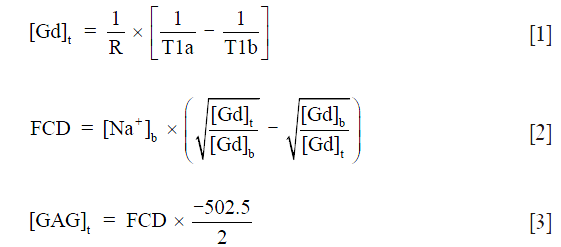
where [Gd]_t is the Gd concentration in the tissue; R is the relaxivity of the Gd ions; T1a and T1b are the T1 values after and before equilibration with Gd, respectively; [Na⁺]_b is the bathing sodium concentration; FCD and [GAG]_t is the fixed charge density and the GAG concentration in the tissue, respectively; the “−2” and “502.5” assumes that there are 2 mols of negative charge per mol of disaccharide with a molecular weight of 502.5 g/mol. Both R value (R =5.77) and T1b value (T1b =1.456 s) were kept constant for the GAG calculations. All µMRI experiments were performed within five days after sacrifice.

µCT experiments

The µCT experiments used a SkyScan 1174 system (Bruker, Kontich, Belgium) with the following imaging parameters: 40 kV, 110 mA, 5 averages, 0.3° rotation step, 180° rotation, 0.2 mm Al filter, and 652 × 512 data matrix per image. Approximately 608 images were acquired for each specimen, which were used to construct a 3D image at an isotropic voxel size of 13.4 µm. All reconstructions used the commercial software NRecon (Bruker, Kontich, Belgium) with the same parameters, where a global intensity threshold was fixed for all scans to include the full range of attenuation values from the cartilage. The scans were converted from gray values to Hounsfield units (HU) based on the properties of air (−1,000 HU) and water (0 HU) (39):

The µCT scans used the blocks ii in Figure 1C and were carried out before (‘baseline’) and after [ioxaglate (Hexabrix, Mallinckrodt, MO, USA)] equilibrating the blocks in a solution containing 40% ioxaglate and 60% saline + PI for approximately 24 h. All the µCT experiments were performed within five days after sacrifice. Before each scan, the cartilage block was gently blotted to remove any excess saline or ioxaglate and was placed in a custom made ‘airtight’ holder with a saline-soaked gauze nearby to minimize any evaporation or shrinkage of the cartilage during the scan. The calculation of the GAG concentration used the following conversion of HU to ioxaglate concentration (36):

and both Eqs. [2] and [3], similar as in the µMRI GAG calculation, replacing Gd concentration with the ioxaglate concentration of the bath and in the tissue.

ICP-OES experiments

Four cartilage blocks (blocks iii in Figure 1C) from each tibia were biochemically treated to measure the bulk GAG content using a PerkinElmer Optima 7000DV ICP-OES (Waltham, MA, USA). For each of the 32 measurements, the cartilage was weighed for wet weight after the underlying bone was removed. The tissue was liquefied by concentrated 100 µL HNO₃ overnight and then diluted to 10 mL using deionized water. A calibration curve was measured as well as the saline solution concentration for accuracy and quality control in ICP-OES. The procedure has been documented before in our previous work (17).

Image and data analysis

All cartilage images from before and after equilibration in contrast agents were analyzed using ImageJ (the National Institutes of Health, Bethesda, MA, USA) for image registration to determine a similar region of interest (ROI) for the depth-dependent analysis. The µMRI experiments used the preliminary coronal images to manually find similar imaging ROI and surface alignment for the sagittal T1b and T1a images. The µCT images were examined in 3D space, rotated, and aligned to find a similar ROI for the baseline and ioxaglate images; ten consecutive 2D images were averaged to produce one 2D µCT image for final analysis. The 2D images from both µMRI and µCT experiments used a 10-column (pixel) average from the surface to the bone to obtain 1D depth-dependent profiles. A representative ROI is shown in Figure 2 for the respective techniques, and all the T1 scans were rotated 55º when calculating the depth-dependent profiles. The 1D depth-dependent profiles begin at the articular surface (defined as 0) and end at the subchondral bone (defined as 1). The full-thickness of cartilage is defined as ‘bulk’ and the sub-tissue zones were defined from the articular surface as: SZ is 10%; TZ is 10%; RZ1 is 40%; RZ2 is 40% (25).

Figure 2 µMRI and µCT images of diseased and contralateral cartilage. (A) A representative set of µMRI T1 images from the PMT and IMT locations oriented at 55º, before (T1b) and after (T1a) equilibrating with the Gd contrast agent; (B) a representative set of µCT images from the same locations of PMT and IMT, before (baseline) and after equilibrating with the ioxaglate contrast agent. The black and white rectangles show the representative ROIs for the µMRI and µCT analysis, respectively. The intensity ranges for µMRI T1b and T1a images have a max of 2 and 1 ms, respectively, with 0 as the minimum for both T1 images. The intensity ranges for the µCT images are 1,750 to −500 HU for the baseline images and 3,500 to −500 HU for the ioxaglate images. PMT, posterior medial tibia; IMT, interior medial tibia.

Statistical analysis

All statistical analyses were performed using KaleidaGraph (Synergy, Reading, PA, USA) and JMP (SAS, Cary, NC, USA). The data was calculated as the mean ± standard deviation. Analysis of variance (ANOVA) with Tukey’s post-hoc test was used to find significant differences between the ACLT and contralateral sections for full thickness and GAG for bulk and all sub-tissue zones. Statistical significance was demonstrated when P values were <0.05.

Results

Cartilage images and thickness

Three weeks after ACLT surgery, a varying degree of visual differences could be found on several surfaces of ACLT and contralateral tibias, a representative of which is shown in Figure 1A,B. The total thickness between the ACLT and the contralateral locations did not demonstrate any significant difference from both the µMRI and µCT measurements, shown in Figure 3 and Table 1.

Figure 3 The bar graphs that compare the ACLT (black) and contralateral (gray) specimens for the µMRI and µCT data, showing the total thickness, the bulk GAG, the SZ GAG, the TZ GAG, the RZ1 GAG, and the RZ2 GAG. The stars mark the locations where a statistical significance between the ACLT and contralateral cartilage has been found. Contra, contralateral; ACLT, anterior cruciate ligament transection; GAG, glycosaminoglycans; SZ, superficial zone; TZ, transitional zone; RZ, radial zone.

Table 1 The µMRI, µCT, and ICP-OES results
Full table

Depth-dependent profiles

In the µMRI data, the general trends in the depth-dependent profiles were similar in both ACLT and contralateral specimens. From the articular surface to the cartilage-bone interface, T1b (pre-contrast) decreased, T1a (post-contrast) increased, and GAG increased. The depth-dependent profiles for the PMT and IMT locations are shown in Figure 4A and Figure 4B, respectively. The GAG profiles with the Gd contrast agent exhibited a visible difference between the ACLT and contralateral specimens at the IMT location, but not between these two specimens at the PMT location. The data at the EMT and CMT locations had the similar trends and differences as the IMT and PMT, respectively (the profiles not shown; the zonal data summarized in Table 1).

Figure 4 The µMRI depth-dependent profiles of T1b, T1a, and GAG concentration for PMT (A) and IMT (B), respectively. The profiles are plotted in a relative depth where the articular surface is denoted as 0 and the bone is 1. The solid circles represent ACLT specimens and the open squares represent the contralateral specimens. The error bars are the standard deviations. Contra, contralateral; GAG, glycosaminoglycans; PMT, posterior medial tibia; IMT, interior medial tibia; ACLT, anterior cruciate ligament transection.

In the µCT data, similar trends as in µMRI were observed between the PMT and IMT specimens (as well as between the EMT and CMT specimens, not shown). From the articular surface to the cartilage-bone interface, the pre-contrast profiles measured similar X-ray attenuations between ACLT and contralateral cartilage at both PMT and IMT locations (Figure 5). The GAG profiles with the use of the contrast agent, however, exhibited a visible difference between the ACLT and contralateral cartilage at the IMT location, but not between these two specimens at the PMT location (Figure 5). The data at the EMT and CMT locations demonstrated similar trends and differences as the IMT and PMT, respectively (profiles not shown; zonal data summarized in Table 1).

Figure 5 The µCT depth-dependent profiles of the baseline, ioxaglate, and GAG concentration for PMT (A) and IMT (B), respectively. The profiles are plotted in a relative depth where the articular surface is denoted as 0 and the bone is 1. The solid circles represent the ACLT specimens and the open squares represent the contralateral specimens. The error bars are the standard deviations. Contra, contralateral; GAG, glycosaminoglycans; PMT, posterior medial tibia; IMT, interior medial tibia; ACLT, anterior cruciate ligament transection.

Thickness and GAG concentrations

Table 1 summarizes the total tissue thickness as well as the zonal averaged GAG concentrations for all four topographical locations on the medial tibial surface (EMT, PMT, CMT, IMT). Some of the comparisons in the Table 1 are plotted in Figure 3 as the bar diagrams. Several trends could be clearly identified:

• The total thickness of the tibial cartilage was location-dependent, topographically. In our canine specimens, the thickness increased from EMT to PMT to CMT to IMT. There was no statistical difference between the ACLT and the contralateral cartilage at the same topographical location (EMT P=0.101, 0.278; PMT P= 0.916, 0.541; CMT P=0.671, 0.271; IMT P=0.597, 0.221) for µMRI and µCT measurements, respectively; both ACLT and contralateral cartilage had the same trend of topographical increment, by both methods (µMRI and µCT);
• The bulk GAG showed a significant increase from the ACLT cartilage to the contralateral cartilage for both EMT and IMT locations on the tibia, by both µMRI and µCT methods. The bulk GAG in the other two locations (PMT and CMT) also showed an increase from the ACLT to contralateral cartilage; but the differences were not statistically significant. Note that the EMT and IMT locations were also the thinnest and the thickest cartilage on the tibia;
• The bulk GAG from the non-imaging ICP-OES measurement demonstrated a significant difference between the ACLT and contralateral cartilage for the EMT, CMT, and IMT locations; but not the PMT locations;
• The zonal GAG showed consistent statistically significant differences between the ACLT and contralateral cartilage, at both EMT and IMT locations, by both µMRI and µCT, for the middle tissue (TZ and RZ1). µCT also showed a statistically significant difference between the two kinds of cartilage in the SZ at the IMT location; while µMRI showed statistical differences between the ACLT and contralateral cartilage in the deepest cartilage (RZ2) at the EMT and IMT locations.

Discussion

This study investigated early degradation in canine cartilage only 3 weeks after the animals underwent an ACLT surgery. The full-thickness ACLT damaged cartilage was slightly less than the contralateral cartilage for almost every location by both µMRI and µCT. The GAG concentration in cartilage was quantified in both high-resolution µMRI and µCT, which were correlated with the biochemical method ICP-OES. A number of significant differences between the ACLT and contralateral cartilage were found in this study, which were both topographical and zonal dependent.

Pre-contrast µMRI and µCT

Although not all individual blocks were scanned for T1b relaxation times in µMRI due to time constraint, two blocks per each topological location were scanned to investigate the effect of Gd on the difference between the ACLT and contralateral cartilage. The depth-dependent T1b relaxation times without the use of Gd contrast agent were found to be independent of the early degradation (Figure 4). T1b were also found to have slight but insignificant differences among topographical locations in the medial tibia. In clinical setting, Trattnig et al. (40) demonstrated that the T1b scan was not necessary in the evaluation of healthy and repaired tissue. In this study, since the R value in Eq. [1] is not routinely measurable in the clinics, a constant R value was used to obtain better alignment with the clinical situation.

In the µCT experiments, the baseline X-ray attenuation (without the use of a contrast agent) was found to be indifferent for all topographical locations in the medial tibia and between the ACLT and contralateral cartilage. This observation confirmed the difficulty in the detection of a cartilage lesion without the contrast agent, because of the low attenuation of X-rays in soft tissues (34,41). It should be noted that the baseline attenuation in CT could measure some other properties of cartilage (e.g., cartilage thickness) and the bone structure (e.g., porosity, bone mineral density) (31,42).

Post-contrast µMRI and µCT

The post-contrast T1 relaxation time (T1a) was found to be lower in the EMT and IMT locations of the ACLT cartilage than the contralateral cartilage, and not markedly different in the PMT and CMT locations of both types of cartilage. This reduction in T1a reflects an increased Gd concentration, indicating a reduced FCD that can be linked to the reduction of the GAG concentration in cartilage. It should be pointed out that the cartilage specimens in this ex vivo µMRI study were kept at ~55° to minimize the dipolar interaction and a stable equilibration was maintained in the ex vivo specimens. Clinically, it would be difficult to orient any joint surface consistently to the magic angle; however, T1 relaxation has been found to be isotropic in cartilage, hence the tissue orientation plays little role in the T1 experiment (38). A second issue between ex vivo and in vivo imaging is that a stable equilibration would be difficult to maintain in any living subject, hence different influx and retreat of the Gd ions could affect an accurate quantification of the GAG concentration in cartilage.

The post-contrast µCT measurement with the use of the ioxaglate attenuation showed an increase for EMT and IMT locations of the ACLT cartilage than the contralateral cartilage, and no difference in the PMT and CMT locations between the ACLT and contralateral cartilage. There was a significant increase in attenuation with the use of the contrast agent, which can be used to improve the detection of cartilage lesion (43). This study shows that high resolution fast imaging with µCT can quantitatively measure the GAG over topographical locations in ex vivo cartilage. A recent work also showed the use of µCT to determine GAG in both in vivo and ex vivo cartilage based upon time-dependent equilibria of a contrast agent (44). The potential for human diagnosis in clinics has been demonstrated (45,46).

GAG concentration

The two imaging techniques measured consistent GAG loss from the ACLT compared to the contralateral cartilage shown in Table 1. Both µMRI and µCT found significant differences in the EMT and IMT locations for the bulk GAG. The µMRI measured increased bulk GAG compared to the µCT results for the EMT and IMT locations but less GAG for the PMT and CMT locations. The biochemical assay found the bulk GAG to be slightly less compared to the imaging techniques. The use of the different contrast agents and techniques showed comparable GAG measurements but each technique could have different sensitivities towards the measured GAG, which could explain some of the differences as well as topographical GAG differences. The depth-dependent GAG measurements using both imaging techniques found significant differences in the TZ and RZ1 for the EMT and IMT locations which could be an indicator of where the cartilage initially degrades. Since the SZ and RZ have the most organized fibers, the GAG could be better constrained than among the more random fibers in the TZ and RZ1.

Recently, Lee et al. (47) investigated topographically the healthy medial tibia plateau and found that the meniscus covered region (EMT and PMT) contained a larger bulk GAG concentration than the uncovered region (IMT and CMT). Compared to the healthy cartilage, the bulk GAG values in the contralateral locations of the covered regions decreased, while the GAG in the uncovered regions did not show much change. In this study, all three techniques found a decrease in GAG in the ACLT cartilage compared with the contralateral cartilage, at all topographical locations in medial tibia; two locations had statistical significant difference among all three techniques and one additional location was significant in ICP-OES measurement. These observations show that there is a detectable GAG loss at the initial stage of cartilage disease—as early as 3 weeks after the ACLT surgery. These observations support the idea that GAG loss is one of the very first signs of OA, which is also characterized later by the loss of collagen integrity (13). The differences in these molecule-level markers have the potential to reveal how the tissue reacts to trauma/injury both topographically and time-dependently. The complementary nature of our three separate modalities could help to differentiate the mechanisms in the disease progression and allow future correlation from bench to bedside.

ACLT surgery

The Pond-Nuki model of OA in canines is likely the most studied large animal model of OA (6,8,10), which have been shown to have the closest similarities with human OA (5). After the ACL has been transected, the stifle subluxation increases the gait irregularity of the joint, which can induce a number of tissue degradation, such as inflammation and surface damage. The damage has been shown to occur over the whole ACLT stifle, including the medial and lateral parts of the tibia and the femur as well as the patella. After the ACL destabilization, the medial compartment has been shown to manifest larger/earlier damage than the lateral compartment (48). To the best of our knowledge, this is the first multi-disciplinary microscopic quantitative imaging study that quantifies the topographical and depth-dependent GAG concentration across the medial plateau only 3 weeks after the ACLT surgery (10,11).

Limitations

In this project, the sample size was limited by the difficulties in investigating a large number of animals and statistical power could be further increased with access to larger sample sizes in future studies. The topographical positions were manually sectioned from the tibias and placed in the coil, which could vary slightly for each different tibia. However, for each topographical location in µMRI, the pre- and post-contrast positions were close to be identical, by imaging the sample in the same slice plane (by taking the coronal pilot images of the blocks).

In conclusion, three independent and complementary techniques were able to quantitatively measure the GAG loss topographically across the medial tibia plateau in canines only 3 weeks after the ACLT surgery. Two different contrast agents were used in two different imaging techniques, which produced consistent results. The ability for these techniques to quantitatively measure the depth-dependent and topographical varying GAG concentration in OA cartilage allows for future investigations that could lead to better understanding and ultimately a better monitoring regarding how OA develops and how it affects the cartilage and other tissues in a joint.

Acknowledgements

The authors are indebted to Dr. John Matyas for performing the ACLT surgeries. The authors are appreciative to Dr. Nian Wang for µMRI expertise. The authors thank Mr. Farid Badar and Dr. Ji-Hyun Lee for help in planning the µMRI experiments.

Funding: The authors are grateful for the National Institutes of Health (NIH) for the support from a R01 grant (AR052353; PI: Y Xia).

Footnote

Conflicts of Interest: The authors have no conflicts of interest to declare.

Ethical Statement: The study was approved by institutional review board at University of Calgary on March 10, 2007, with an animal welfare assurance number of A5018-01 and written informed consent was obtained from all patients.

References

1. Venn M, Maroudas A. Chemical composition and swelling of normal and osteoarthrotic femoral head cartilage. I. Chemical composition. Ann Rheum Dis 1977;36:121-9. [Crossref] [PubMed]
2. Mittelstaedt D, Xia Y, Shmelyov A, Casciani N, Bidthanapally A. Quantitative determination of morphological and territorial structures of articular cartilage from both perpendicular and parallel sections by polarized light microscopy. Connect Tissue Res 2011;52:512-22. [Crossref] [PubMed]
3. Maroudas AI. Balance between swelling pressure and collagen tension in normal and degenerate cartilage. Nature 1976;260:808-9. [Crossref] [PubMed]
4. Buckwalter JA, Mankin HJ, Grodzinsky AJ. Articular cartilage and osteoarthritis. Instr Course Lect 2005;54:465-80. [PubMed]
5. McCoy AM. Animal Models of Osteoarthritis: Comparisons and Key Considerations. Vet Pathol 2015;52:803-18. [Crossref] [PubMed]
6. Pond MJ, Nuki G. Experimentally-induced osteoarthritis in the dog. Ann Rheum Dis 1973;32:387-8. [Crossref] [PubMed]
7. Marijnissen AC, van Roermund PM, TeKoppele JM, Bijlsma JW, Lafeber FP. The canine 'groove' model, compared with the ACLT model of osteoarthritis. Osteoarthritis Cartilage 2002;10:145-55. [Crossref] [PubMed]
8. Libicher M, Ivancic M, Hoffmann M, Wenz W. Early changes in experimental osteoarthritis using the Pond-Nuki dog model: technical procedure and initial results of in vivo MR imaging. Eur Radiol 2005;15:390-4. [Crossref] [PubMed]
9. Visco DM, Hill MA, Widmer WR, Johnstone B, Myers SL. Experimental osteoarthritis in dogs: a comparison of the Pond-Nuki and medial arthrotomy methods. Osteoarthritis Cartilage 1996;4:9-22. [Crossref] [PubMed]
10. Alhadlaq HA, Xia Y, Moody JB, Matyas JR. Detecting structural changes in early experimental osteoarthritis of tibial cartilage by microscopic magnetic resonance imaging and polarised light microscopy. Ann Rheum Dis 2004;63:709-17. [Crossref] [PubMed]
11. Lee JH, Badar F, Kahn D, Matyas J, Qu X, Xia Y. Loading-induced changes on topographical distributions of the zonal properties of osteoarthritic tibial cartilage--A study by magnetic resonance imaging at microscopic resolution. J Biomech 2015;48:3625-33. [Crossref] [PubMed]
12. Pritzker KP, Gay S, Jimenez SA, Ostergaard K, Pelletier JP, Revell PA, Salter D, van den Berg WB. Osteoarthritis cartilage histopathology: grading and staging. Osteoarthritis Cartilage 2006;14:13-29. [Crossref] [PubMed]
13. Lee JH, Badar F, Matyas J, Qu X, Xia Y. Topographical variations in zonal properties of canine tibial articular cartilage due to early osteoarthritis: a study using 7-T magnetic resonance imaging at microscopic resolution. MAGMA 2016;29:681-90. [Crossref] [PubMed]
14. Tiderius CJ, Olsson LE, Leander P, Ekberg O, Dahlberg L. Delayed gadolinium-enhanced MRI of cartilage (dGEMRIC) in early knee osteoarthritis. Magn Reson Med 2003;49:488-92. [Crossref] [PubMed]
15. Eckstein F, Burstein D, Link TM. Quantitative MRI of cartilage and bone: degenerative changes in osteoarthritis. NMR Biomed 2006;19:822-54. [Crossref] [PubMed]
16. Taylor C, Carballido-Gamio J, Majumdar S, Li X. Comparison of quantitative imaging of cartilage for osteoarthritis: T2, T1rho, dGEMRIC and contrast-enhanced computed tomography. Magn Reson Imaging 2009;27:779-84. [Crossref] [PubMed]
17. Wang N, Chopin E, Xia Y. The effects of mechanical loading and gadolinium concentration on the change of T1 and quantification of glycosaminoglycans in articular cartilage by microscopic MRI. Phys Med Biol 2013;58:4535-47. [Crossref] [PubMed]
18. Wang YX, Wang J, Deng M, Liu G, Qin L. In vivo three-dimensional magnetic resonance imaging of rat knee osteoarthritis model induced using meniscal transection. J Orthop Translat 2015;3:134-41. [Crossref]
19. Silvast TS, Kokkonen HT, Jurvelin JS, Quinn TM, Nieminen MT, Töyräs J. Diffusion and near-equilibrium distribution of MRI and CT contrast agents in articular cartilage. Phys Med Biol 2009;54:6823-36. [Crossref] [PubMed]
20. Maroudas A. Distribution and diffusion of solutes in articular cartilage. Biophys J 1970;10:365-79. [Crossref] [PubMed]
21. Torzilli PA, Arduino JM, Gregory JD, Bansal M. Effect of proteoglycan removal on solute mobility in articular cartilage. J Biomech 1997;30:895-902. [Crossref] [PubMed]
22. Xia Y, Farquhar T, Burton-Wurster N, Vernier-Singer M, Lust G, Jelinski LW. Self-diffusion monitors degraded cartilage. Arch Biochem Biophys 1995;323:323-8. [Crossref] [PubMed]
23. Nieminen MT, Rieppo J, Silvennoinen J, Töyräs J, Hakumäki JM, Hyttinen MM, Helminen HJ, Jurvelin JS. Spatial assessment of articular cartilage proteoglycans with Gd-DTPA-enhanced T1 imaging. Magn Reson Med 2002;48:640-8. [Crossref] [PubMed]
24. Kulmala KA, Korhonen RK, Julkunen P, Jurvelin JS, Quinn TM, Kröger H, Töyräs J. Diffusion coefficients of articular cartilage for different CT and MRI contrast agents. Med Eng Phys 2010;32:878-82. [Crossref] [PubMed]
25. Xia Y, Moody JB, Burton-Wurster N, Lust G. Quantitative in situ correlation between microscopic MRI and polarized light microscopy studies of articular cartilage. Osteoarthritis Cartilage 2001;9:393-406. [Crossref] [PubMed]
26. Lesperance LM, Gray ML, Burstein D. Determination of fixed charge density in cartilage using nuclear magnetic resonance. J Orthop Res 1992;10:1-13. [Crossref] [PubMed]
27. Bashir A, Gray ML, Burstein D. Gd-DTPA2- as a measure of cartilage degradation. Magn Reson Med 1996;36:665-73. [Crossref] [PubMed]
28. Gillis A, Gray M, Burstein D. Relaxivity and diffusion of gadolinium agents in cartilage. Magn Reson Med 2002;48:1068-71. [Crossref] [PubMed]
29. Xia Y, Zheng S, Bidthanapally A. Depth-dependent profiles of glycosaminoglycans in articular cartilage by microMRI and histochemistry. J Magn Reson Imaging 2008;28:151-7. [Crossref] [PubMed]
30. Zheng S, Xia Y. The impact of the relaxivity definition on the quantitative measurement of glycosaminoglycans in cartilage by the MRI dGEMRIC method. Magn Reson Med 2010;63:25-32. [PubMed]
31. McErlain DD, Appleton CT, Litchfield RB, Pitelka V, Henry JL, Bernier SM, Beier F, Holdsworth DW. Study of subchondral bone adaptations in a rodent surgical model of OA using in vivo micro-computed tomography. Osteoarthritis Cartilage 2008;16:458-69. [Crossref] [PubMed]
32. Piscaer TM, Waarsing JH, Kops N, Pavljasevic P, Verhaar JA, van Osch GJ, Weinans H. In vivo imaging of cartilage degeneration using microCT-arthrography. Osteoarthritis Cartilage 2008;16:1011-7. [Crossref] [PubMed]
33. Bansal PN, Joshi NS, Entezari V, Grinstaff MW, Snyder BD. Contrast enhanced computed tomography can predict the glycosaminoglycan content and biomechanical properties of articular cartilage. Osteoarthritis Cartilage 2010;18:184-91. [Crossref] [PubMed]
34. Palmer AW, Guldberg RE, Levenston ME. Analysis of cartilage matrix fixed charge density and three-dimensional morphology via contrast-enhanced microcomputed tomography. Proc Natl Acad Sci U S A 2006;103:19255-60. [Crossref] [PubMed]
35. Yoo HJ, Hong SH, Choi JY, Lee IJ, Kim SJ, Choi JA, Kang HS. Contrast-enhanced CT of articular cartilage: experimental study for quantification of glycosaminoglycan content in articular cartilage. Radiology 2011;261:805-12. [Crossref] [PubMed]
36. Mittelstaedt D, Xia Y. Depth-Dependent Glycosaminoglycan Concentration in Articular Cartilage by Quantitative Contrast-Enhanced Micro-Computed Tomography. Cartilage 2015;6:216-25. [Crossref] [PubMed]
37. Xia Y. Relaxation anisotropy in cartilage by NMR microscopy (muMRI) at 14-microm resolution. Magn Reson Med 1998;39:941-9. [Crossref] [PubMed]
38. Xia Y. Magic-angle effect in magnetic resonance imaging of articular cartilage: a review. Invest Radiol 2000;35:602-21. [Crossref] [PubMed]
39. Hounsfield GN. Computed medical imaging. Nobel lecture, Decemberr 8, 1979. J Comput Assist Tomogr 1980;4:665-74. [Crossref] [PubMed]
40. Trattnig S, Burstein D, Szomolanyi P, Pinker K, Welsch GH, Mamisch TC. T1(Gd) gives comparable information as Delta T1 relaxation rate in dGEMRIC evaluation of cartilage repair tissue. Invest Radiol 2009;44:598-602. [Crossref] [PubMed]
41. Xie L, Lin AS, Levenston ME, Guldberg RE. Quantitative assessment of articular cartilage morphology via EPIC-microCT. Osteoarthritis Cartilage 2009;17:313-20. [Crossref] [PubMed]
42. Anderson AE, Ellis BJ, Peters CL, Weiss JA. Cartilage thickness: factors influencing multidetector CT measurements in a phantom study. Radiology 2008;246:133-41. [Crossref] [PubMed]
43. Kokkonen HT, Jurvelin JS, Tiitu V, Töyräs J. Detection of mechanical injury of articular cartilage using contrast enhanced computed tomography. Osteoarthritis Cartilage 2011;19:295-301. [Crossref] [PubMed]
44. Hirvasniemi J, Kulmala KA, Lammentausta E, Ojala R, Lehenkari P, Kamel A, Jurvelin JS, Töyräs J, Nieminen MT, Saarakkala S. In vivo comparison of delayed gadolinium-enhanced MRI of cartilage and delayed quantitative CT arthrography in imaging of articular cartilage. Osteoarthritis Cartilage 2013;21:434-42. [Crossref] [PubMed]
45. Siebelt M, van Tiel J, Waarsing JH, Piscaer TM, van Straten M, Booij R, Dijkshoorn ML, Kleinrensink GJ, Verhaar JA, Krestin GP, Weinans H, Oei EH. Clinically applied CT arthrography to measure the sulphated glycosaminoglycan content of cartilage. Osteoarthritis Cartilage 2011;19:1183-9. [Crossref] [PubMed]
46. van Tiel J, Siebelt M, Waarsing JH, Piscaer TM, van Straten M, Booij R, Dijkshoorn ML, Kleinrensink GJ, Verhaar JA, Krestin GP, Weinans H, Oei EH. CT arthrography of the human knee to measure cartilage quality with low radiation dose. Osteoarthritis Cartilage 2012;20:678-85. [Crossref] [PubMed]
47. Lee JH, Badar F, Kahn D, Matyas J, Qu X, Chen CT, Xia Y. Topographical variations of the strain-dependent zonal properties of tibial articular cartilage by microscopic MRI. Connect Tissue Res 2014;55:205-16. [Crossref] [PubMed]
48. Dejour H, Bonnin M. Tibial translation after anterior cruciate ligament rupture. Two radiological tests compared. J Bone Joint Surg Br 1994;76:745-9. [PubMed]