
Image-spectral decomposition extended-learning assisted by sparsity for multi-energy computed tomography reconstruction
Introduction
Multi-energy computed tomography (CT) has huge potentials in material identification, tissue characterization and metal artifacts reduction (1). Due to the lower costs and more flexible implementation, dual-energy CT (DECT) has been applied to different clinical applications (2,3). In principle, DECTs are the most predominant approaches for accurately reconstructing two basis materials by providing two distinct energy windows. Yet, many clinical and industrial applications require three or more basis material images (4). The currently available DECT system uses either dual-source with dual-detector, dual-layer detectors, or switchable dual sources (5). However, the detector is still energy-integrating. It results in significant spectral overlap and subjects to spectral blurring. Compared with DECT, the state-of-the-art photon-counting detector (PCD) based multi-energy CT has remarkably higher distinguishability. The PCD hardware usually employs a semiconductor sensor (e.g., CdTe, CdZnTe) to capture the energy information from the transmitted X-ray spectrum passing through materials. Thus, PCD based multi-energy CT can sample more data points from a single exposure without additional radiation dose for image reconstruction and multi-material decomposition. In addition, the beam hardening artifacts and spectrum overlap between the multi-energy images are minimized. With these unique advantages, the multi-energy CT technologies can provide abundant spectral-spatial characteristics, which significantly improves the quality of reconstructed channel-wise images and the accuracy of material decomposition map (6). Hence, multi-energy CT plays a critical role in numerous applications such as K-edge imaging (7), low-dose CT (8), and material decomposition (9). Nevertheless, there are still some drawbacks to be solved for multi-energy CT, such as the quantum noise, charge sharing and pulse pileup effects. These factors can lead to lower signal-noise-ratio (SNR) projection datasets, compromising multi-energy images and material decomposition accuracy. How to reconstruct high-quality images has been of great interest for multi-energy CT in recent years. To overcome these difficulties, some researchers focus on developing more mature higher-powered PCDs (10). Others pay attention to proposing effective multi-energy CT image reconstruction models to suppress the noisy artifacts. In this work, we will develop advanced reconstruction algorithms.
Multi-energy CT images have local sparsity, nonlocal self-similarity in spatial dimension and correlation in spectral dimension. The local sparsity is inherited from traditional CT image, the correlation property is based on the similarity between multi-energy bin images, and the nonlocal self-similarity is based on many similar image patches. To utilize those intrinsic priors, various multi-energy CT reconstruction models have been proposed. Early multi-energy CT reconstruction algorithms usually used two-dimensional (2D) methods to reconstruct single energy images individually. Following this strategy, several studies have been reported. For example, Xu et al. (11) adopted a total variation (TV) regularization to multi-energy CT. Meantime, a vector-based dual-dictionary learning (DL) method was reported in (12). Zhang et al. proposed a TV-TV and TV spectral mean model to improve the multi-energy CT images in (13). However, such algorithms are unsatisfactory because they only consider local sparsity and ignore the intrinsic correlation priors. To tackle this issue, Wang et al. adopted a high-quality full-spectrum prior image as a supervision information to optimize the multi-energy CT reconstruction images (14). Meanwhile, to obtain narrow energy bin images with lower noise, Yu et al. applied the prior image constrained compressed sensing (PICCS) framework to photon-counting CT, generating the spectral PICCS (SPICCS) (15,16). Although these channel-wise reconstruction methods exploit both local sparsity and the correlation priors to a certain degree, they take a great deal of time to optimize the parameters in practice due to the large number of energy bins.
To jointly consider the correlation and nonlocal self-similarity information for multi-energy CT reconstruction, low rank (LR) regularization and tensor-based processing methods were introduced to multi-energy CT (4). In (17), a LR constraint is introduced to multi-energy CT reconstruction. Gao et al. proposed a prior rank, intensity and sparsity model (PRISM) (18) by modeling spectral images as the superposition of a low-rank matrix and a sparse matrix. Semerci et al. combined the tensor-based nuclear norm (TNN) and TV regularizations for multi-energy CT (19). Tensor dictionary learning (TDL) was developed in (20) by considering the advantages of DL in sparse representation. Later in (21), encouraged by the advantages in edge preservation, the image gradient L0-norm regularization was introduced to TDL model for low-dose multi-energy CT (22). Moreover, a spectral-image similarity-based tensor with enhanced-sparsity (SISTER) method was proposed in (23). Meanwhile, a spatial-spectral cube matching frame (SSCMF) method was proposed (24). Then, to address the limitation of SSCMF, Wu et al. proposed a non-local low-rank cube-based tensor factorization (NLCTF) method (25).
However, the NLCTF still has some limitations. First, the cube extraction and aggregation operation methods in the NLCTF algorithm can result in the inconsistency issue of the overlapped pixels and increase the computational complexity per iteration. Second, the DL aims to find a set of atoms for a given patch-wise training dataset, where each patch can be represented by a few of these atoms. By using a well-trained dictionary, noise can be effectively removed. However, the NLCTF does not contain a DL component, which means the NLCTF does not fully code the intrinsic correlation and nonlocal self-similarity priors. Third, NLCTF mainly focuses on exploring the correlation and nonlocal self-similarity priors by formulating low-rank model, and the local sparsity property of single energy-bin image is relaxed.
To address these problems of NLCTF and fully utilize the local sparsity, correlation and nonlocal self-similarity priors in multi-energy CT images, in this work, we propose an image-spectral decomposition extended-learning assisted by sparsity (IDEAS) algorithm for multi-energy CT image reconstruction. As shown in the flowchart in Figure 1, first, a nonlocal low-rank Tucker tensor decomposition model is proposed based on the inherent correlation and nonlocal self-similarity regularizers. Compared to the whole multi-energy images, the rank of similar patch group is much lower, and therefore, to simplify the computational complexity, we use the k-means++ clustering method to explore the nonlocal self-similarity property. Second, inspired by the advantages of TDL in sparse representation, the multi-task DL is employed in terms of an adaptive spatial dictionary and an adaptive spectral dictionary which are trained during an iterative reconstruction process. Third, a weighted TV regularization term is employed to encourage local sparsity of single energy-bin image. Due to the good capabilities of noise suppression and edge preservation of image-domain material decomposition method, we consider a linear assumption and use an image-domain material decomposition method to obtain high-quality basis material images.
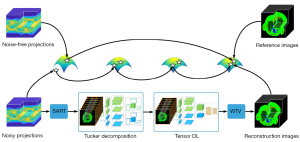
The main contributions of this paper are listed as follow. First, IDEAS method is developed to fully encode the local sparsity, correlation and nonlocal self-similarity properties of multi-energy CT images by combining multiple regularizations, including non-local low-rank Tucker decomposition, TDL and weighted TV. Second, an effective split-Bregman technique is developed to optimize the IDEAS algorithm. Third, numerical experiments on numerical simulations and physical phantom experiments show that the proposed IDEAS method reaches better performance than the state-of-the-art algorithms in terms of qualitative and quantitative measurements. In addition, IDEAS model can be used for multi-spectral image denoising and dynamic magnetic resonance imaging.
Methods
Multi-energy CT imaging model
Multi-energy CT provides several sets of projections simultaneously by dividing X-ray spectrum into different energy channels with appropriate post-processing steps. Considering the noise in projections, the forward model for fan-beam geometry can be expressed as a linear system:
where denote the multi-energy CT projections and is desired multi-energy images, S denotes the number of energy bins, is the sinogram for sth energy bin, T1 and T2 represent the numbers of view and detector element and their product equals to T, is the image reconstructed from the sth energy bin sinogram, I1 and I2 represent the height and width and their product equals to I, M is a linear system operator to map the image tensor to projection tensor, and is the noise term. To recover the object image, we can solve the following minimization problem:
where represents the square of Frobenius norm. Here, Eq. [2] can be minimized by the algebraic reconstruction technique (ART) or simultaneous algebraic reconstruction technique (SART) methods. In practical applications, Eq. [2] is an ill-posed inverse problem, and a common strategy is to incorporate regularization term(s) (26). Hence, we have
where the first term represents data fidelity, the second term represents the regularization function, and δ>0 is regularization parameter to control constraint intensity.
Multidimensional DL
On one hand, small image patches of a medical imaging object usually contain only 1–2 materials. This means that the image patch has lower rank than the whole images. On the other hand, the nonlocal self-similarity property refers to the fact that small patches among different locations share similar structural information. Moreover, these small image patches can form a high-quality training set to enhance the image quality of DL reconstruction. Similar to our previous work (27), for a multi-energy CT image , let us define a extracting, k-means++ clustering (28), and unfolding operator is . We can obtain a series of similar tensor patch groups , where is the tensor group of Ω, are the size of extracted patches, Il is the number of similar patches. Considering a tensor training set extracted from the tensor image . Here, we set each reconstructed tensor group as a sparse representation of a spatial dictionary , a spectral dictionary , where and are redundancy ratios corresponding to the spatial dictionary and the spectral dictionary, respectively. Then, we have
where is the sparse coefficient tensor of the reconstructed tensor group, ×n is the n-mode product of a tensor with a matrix, and ql restricts the number of non-zero elements. is the sparse constraint, and and are normalization constraints. Then, Eq. [4] can be further converted into another constrained minimization problem
where δ1>0 is an empirical parameter.
Tucker low-rank tensor decomposition
Tensor decomposition has been widely used in signal processing, computer vision and machine learning, etc. Generally, a tensor can be decomposed as the summation of rank-1 tensors, the number of the rank-1 tensor is called tensor rank. There are different forms of tensor rank with respect to different tensor decomposition methods, such as canonical polyadic (CP) decomposition (29), Tucker decomposition (30), t-singular value decomposition (SVD) (31), and kronecker-basis-representation (KBR)-based tensor decomposition (32), etc.
As one of the most popular tensor decomposition methods, the Tucker decomposition is a generalization of matrix SVD in high dimensional space, which is flexible and computationally tractable (33). For the 3rd-order tensor groups , the Tucker decomposition can be expressed as
where “T” represents the matrix transpose, is a core tensor, and are factors. The optimization problem in Eq. [6] is convex and can be solved by higher-order singular value decomposition (HOSVD) (34) or higher-order orthogonal iteration (HOOI) (35).
Weighted TV regularization
Considering the local sparsity of multi-energy CT images, we introduce the TV regularization (36,37) to enhance the reconstructed image tensor . The conventional isotropic TV regularization is specifically designed to handle 2D images. Because the multi-energy CT contains several energy bins, the photon energies of different channels are different, the corresponding material attenuation coefficients are different, and scales of channel-wise image are different. To obtain high-quality channel-wise images, it is necessary to provide different parameters for different channels. That needs high computational cost to deal with the parameters in practice with the conventional TV. To address this problem, a weighting factor ws is introduced to the TV regularization, leading to a weighted TV regularization. This can be denoted as
where and represent the values of image gradient along height and width directions in spatial mode.
IDEAS model and solution
Encouraged by the aforementioned facts, here we combine multiple regularizations, including non-local low-rank Tucker tensor decomposition, TDL and weighted TV, for multi-energy CT reconstruction. Our proposed reconstruction model of IDEAS can be formulated as
where and are three regularization factors. To efficiently handle the L1-norm and optimize the objective function Eq. [8], the split-Bregman method is utilized in this study (38). L auxiliary tensors , ν and the corresponding feedback error tensors , are introduced into Eq. [8]. Then we have
where and are two coupling parameters, which are to balance two regularizes. Because Eq. [9] contains multiple variables, we can further divide it several subproblems by fixing other variables and removing the irrelevant terms.
Updating
where is the iterative index. Eq. [10] is differentiable and could be directly solved by the gradient descent method.
where β is a relaxation factor (27), is the inverse operation of .
Updating
Noting that each group is independent, and we have
Defining with the symbol “” as Kronecker product of matrices, Eq. [12] can be solved by gradient descent method. The solution is
where I is an identity matrix, are unfolding the in the 3rd mode. Therefore, tensor can be obtained by folding at the 3rd mode. More details about updating is given in Appendix 1.
Updating
This leads to a closed-form solution in terms of soft-thresholding filtering
where denotes the soft-thresholding operator. Then, can be given by derivative decent method directly.
Updating D1 and D2
Because two dictionaries are shared by all groups, by using , the optimization problem is involved into
and are obtained by stacking all groups of and at the 3rd-order mode, respectively. Define . Then, we have
where and are unfolding the in the 1st mode. The optimization problem in Eq. [17] is a quadratically constrained quadratic programming problem and can be solved using a Lagrange dual (39). D1 can be updated by
where is diagonal matrix and are dual variables whose values are obtained by solving the dual problem. Similarly, D2 can be obtained.
Updating
In this work, we use HOSVD (34) to solve [19], and we have
are the rank of (40).
Updating
After substituting Eq. [7] into Eq. [9] and removing irrelevant terms, we have
Assuming the amplitude of boundary gradient are zero, for the sth energy bin, Eq. [21] can be further evolved into
where and . Similarly, Eq. [22] is solved by split-Bregman algorithm. More details about updating is given in Appendix 2.
Then, can be given by derivative decent method directly. Till now, we have finished all implementation procedures of the proposed IDEAS method. To make it clear, the pseudocodes of the proposed method are summarized as in Table 1.
Table 1
| IDEAS |
| Input: γ, υ, δ1, ρ, λ, κ1, κ2, η, β; |
| Initialization: ; |
| While not convergence do; |
| Updating using [11]; |
| Constructing groups by extracting, clustering and unfolding process of ; |
| For ; |
| Updating via folding by [13]; |
| Updating using [15]; |
| Updating via derivative decent method; |
| End for |
| Updating using [18]; |
| Updating with step 11; |
| For |
| Updating using [20]; |
| End for |
| Updating using [22]; |
| Updating via derivative decent method; |
| End while |
| Output: |
IDEAS, image-spectral decomposition extended-learning assisted by sparsity.
Results
Numerical mouse simulations, physical phantom and preclinical mouse experiments are performed. The SART, TV (11), TV and LR (TV+LR) (17), SSCMF (24) and NLCTF are also implemented for a comparison study. For all the iterative techniques, the initial images are set as zero and all of them are stopped after 50 iterations. In the implementation, the formulation of a low-rank patch , , and the step size are set as 7, 7, and 5, respectively. The redundancy ratios and are set as 1.5. The size of the corresponding spatial dictionary D1 and spectral dictionary D2 are set as 49×73 and 8×12, respectively. Others parameters () need to be tuned. Specifically, β=0.03 and δ=10 in all experiments. The rest of the parameters are empirically selected by comparing the quantitative indexes in numerical simulation study. In the physical phantom study, we select the parameters based on visual evaluation (including features recovery, detail retain and edge preservation). By using these parameter tuning strategies, all the reconstruction methods reach the best results and the corresponding optimized parameters are listed in Table 2 (The symbols are consistent with the reference).
Table 2
| Methods | Numerical simulation | Physical phantom study |
|---|---|---|
| SART | β=0.03 | β=0.03 |
| TV | γ=0.7, Num =20 | γ=0.2, Num =20 |
| TV+LR | λ1=5, λ2=1/40, μ1=0.1, μ2=0.25 | λ1=1, λ2=1/23, μ1=0.1, μ2=0.02 |
| SSCMF | σ=0.05, τ=10 | σ=0.005, τ=0.4 |
| NLCTF | α=100, τ=0.055, ϑ=250, μ=0.3 | α=10, τ=0.025, ϑ=250, μ=0.5 |
| IDEAS | ν=0.01, ρ=0.01, λ=0.5, κ1=0.01, κ2=38, η=10 | ν=0.005, ρ=0.5, λ=0.25, κ1=0.0005, κ2=30, η=20 |
SART, simultaneous algebraic reconstruction technique; TV, total variation; LR, low rank; SSCMF, spatial spectral cube matching frame; NLCTF, non-local low-rank cube-based tensor factorization; IDEAS, image-spectral decomposition extended-learning assisted by sparsity.
Numerical simulation study
In the numerical tests, a digital thorax mouse phantom with 1.2% injected iodine contrast agent (Figure 2) (41) is employed. A polychromatic 50 kVp X-ray source is assumed, and its spectrum is divided into eight energy bins: [16, 22), [22, 25), [25, 28), [28, 31), [31, 34), [34, 37), [37, 41), and [41, 50) keV. A total of 640 projections are uniformly collected in an equidistant fan-beam geometry, where the distances from the X-ray source to PCD and object are set as 180 and 132 mm, respectively. The PCD system consists of 512 elements and each of them covers a length of 0.1 mm. A total of 5,000 incident photons are assumed for each X-ray path for all the bins, which matched the setup of real Medipix all resolution system (MARS) PCD (42). To generate multi-energy projections, the incident photons were distributed to each energy bin according to the X-ray spectrum (Figure 2). By using fan-beam equal distance projection, we computed the expected number of photons in each bin for every spectral detector element. Then, we first obtained the noise-free projections by a logarithmic operation. To simulate a realistic clinical environment, Poisson noise is superimposed to to obtain the noisy projection , where I0 is the number of photons before the X-rays penetrate the object and the number of photons in 1–8 energy bins are 693, 627, 700, 692, 631, 539, 557, 562, respectively. The reconstructed and decomposed images are with 512×512 pixels. For each pixel, the physical dimension is 0.075×0.075 mm2. The image quality is evaluated in terms of the root mean square error (RMSE), and structural similarity (SSIM) (43).
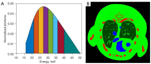
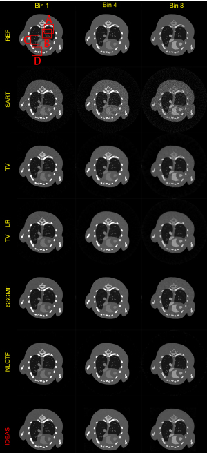
Figure 3 shows the reconstructed results of three representative energy bins (1st, 4th and 8th) by different methods, and the noise-free reference images are obtained by the SART method. Without any prior knowledge, the SART results have heavy noise and severe image artifacts. Although the reconstructed images of TV and TV+LR are improved (3rd and 4th rows) regularized by prior knowledge, they still have blocky artifacts and blurry edges due to the drawbacks of TV regularization. The results of SSCMF and NLCTF methods have better features without blocky artifacts compared with those reconstructed by the TV and TV+LR methods. However, some finer structures are still lost and some edges are still blurry in the SSCMF and NLCTF results. Compared with all the aforementioned methods, the IDEAS provides clear image edges and more image structures.
To clearly show the differences among the reconstructed results of all algorithms, Figure 4 displays magnified regions of interest (ROIs) indicated by the red rectangle in Figure 3. Evidently, the IDEAS method more effectively reduces noise-induced artifacts and obtains more reasonable texture information than other methods. From Figure 4A-4C, one can see that many finer structures and details are disappeared in most reconstructed images. However, they always can be seen in the NLCTF and IDEAS methods. that as the algorithm is updated, the bone structures become clearer and clearer (see the red arrow 8). Although the NLCTF preserves some structures, these structures are blurred. Compared with the NLCTF, we can observe that the IDEAS preserves finer structures and details, and it has better performance in image edge preservation indicated by the arrows “1”, “2”, “4”, “5” and “6”, which are close to the references. Moreover, from Figure 4B,4C, one can see the NCLTF results are tarnished by severe artifacts indicated by arrows “3” and “7”. They make it not easy to discriminate the features and artifacts in some cases. Obviously, the proposed IDEAS algorithm can suppress these artifacts, preserving finer structures and edge information. Table 3 lists the quantitative results of reconstructed images. The SSIM measures the similarity between the reconstructed images and references. The closer to 1.0 the SSIM value is, the better the reconstructed image is. One can see that the presented IDEAS produces the best RMSE and SSIM values for all energy bins, which indicate that IDEAS can yield the best image quality among all the methods for all energy bins. From Table 3, we can see that the quantitative index of the proposed IDEAS algorithm is significantly improved in low energy bins comparing to the NLCTF technique.
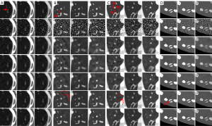
Table 3
| Index | Methods | Reconstructed images (energy bins) | Material decomposition | ||||||||||
|---|---|---|---|---|---|---|---|---|---|---|---|---|---|
| 1st | 2nd | 3rd | 4th | 5th | 6th | 7th | 8th | Bone | Soft tissue | Iodine | |||
| RMSE (10−2) | SART | 32.84 | 23.52 | 18.94 | 17.04 | 16.43 | 16.89 | 15.80 | 14.91 | 3.81 | 18.41 | 13.84 | |
| TV | 10.15 | 6.68 | 5.15 | 4.23 | 3.83 | 3.70 | 3.21 | 2.78 | 2.05 | 6.31 | 4.00 | ||
| TV+LR | 10.00 | 6.16 | 4.55 | 3.62 | 3.12 | 3.31 | 2.80 | 2.40 | 2.15 | 6.35 | 3.84 | ||
| SSCMF | 9.20 | 5.48 | 4.20 | 3.69 | 2.91 | 2.69 | 2.24 | 1.79 | 2.03 | 5.46 | 2.94 | ||
| NLCTF | 8.43 | 5.29 | 3.79 | 2.85 | 2.27 | 2.25 | 1.90 | 1.58 | 1.99 | 4.84 | 2.87 | ||
| IDEAS | 6.72 | 4.31 | 3.16 | 2.39 | 1.95 | 2.00 | 1.65 | 1.36 | 1.52 | 4.16 | 2.41 | ||
| SSIM | SART | 0.5596 | 0.5211 | 0.5038 | 0.4528 | 0.4114 | 0.3545 | 0.3340 | 0.2879 | 0.7164 | 0.3237 | 0.4500 | |
| TV | 0.9533 | 0.9570 | 0.9580 | 0.9512 | 0.9414 | 0.9207 | 0.9109 | 0.8932 | 0.9880 | 0.8355 | 0.8972 | ||
| TV+LR | 0.9525 | 0.9649 | 0.9657 | 0.9608 | 0.9524 | 0.9272 | 0.9209 | 0.9040 | 0.9862 | 0.8141 | 0.9106 | ||
| SSCMF | 0.9666 | 0.9640 | 0.9670 | 0.9649 | 0.9629 | 0.9518 | 0.9460 | 0.9353 | 0.9906 | 0.8829 | 0.9542 | ||
| NLCTF | 0.9751 | 0.9755 | 0.9753 | 0.9742 | 0.9724 | 0.9622 | 0.9598 | 0.9558 | 0.9913 | 0.8749 | 0.9657 | ||
| IDEAS | 0.9810 | 0.9789 | 0.9780 | 0.9775 | 0.9745 | 0.9631 | 0.9617 | 0.9561 | 0.9936 | 0.8911 | 0.9705 | ||
Quantitative testing. RMSE, root mean square error; SSIM, structural similarity; SART, simultaneous algebraic reconstruction technique; TV, total variation; LR, low rank; SSCMF, spatial spectral cube matching frame; NLCTF, non-local low-rank cube-based tensor factorization; IDEAS, image-spectral decomposition extended-learning assisted by sparsity. This table is licensed by IEEE publisher.
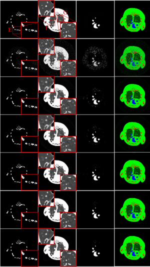
To further demonstrate the advantages of the proposed IDEAS method, an image-domain material decomposition method (44,45) is utilized to decompose the reconstructed results into material-specific images. Specifically, a linear assumption is employed to link the reconstructed channel-wise images with the material images, and a direct inversion (DI) method is employed to obtain final material decomposition results. The decomposition system matrix was obtained by computing the averaged mass coefficients of reconstructed SART images (46). The inaccurately reconstructed images may lead to errors of the decomposition system matrix. Besides, the DI method can yield amplified image noise and have rather big error in the boundary pixels. To address this issue, three additional constraints in terms of the volume conservation (47), the bound of each material pixel ([0, 1]) (48), and the concentration of iodine contrast (no more than 5%) (44) are incorporated into the material model to further improve the final results. Figure 5 shows the corresponding basis materials and the color rendering images of Figure 3. The 1st column of Figure 5 shows the bone component. The bony structures are blurred in the compared algorithms, and IDEAS results produce clear bone edges (see the ROI “E”). Moreover, IDEAS provides more soft-tissue features than the competing methods (see the ROIs “F” and “G”). In terms of iodine contrast component (3rd column), some bony region pixels are wrongly introduced by all the competing methods, while the presented IDEAS performs well. In addition, Table 3 displays the quantitative results of material-specific images. One can see that IDEAS achieves the best RMSE and SSIM values for all the materials. This confirms that the proposed method can provide the most accurate material decomposition images.
The convergences of different methods are also investigated, and the RMSEs of channel 1 image versus iteration number are given in Figure 6. By comparison, the IDEAS can converge to an optimized solution quickly with a smaller RMSE. In addition, for all the reconstruction methods, approximately 30 iterations can produce an acceptable solution. In this case, we set all the iterative methods to stop after 50 iterations. Computational cost is an important factor for the reconstruction algorithm development. In this work, all the algorithms are programmed by Matlab (2019a) on an Intel(R) Core (TM) i9-9920X CPU, 3.70 GHz, PC platform. The computational costs of SART, TV, TV+LR, SSCFM, NLCTF and IDEAS in one iteration are listed in Table 4. Compared with the NLCTF, the presented IDEAS greatly reduces the computational cost.
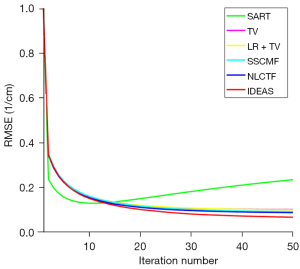
Table 4
| Methods | Costs |
|---|---|
| SART | 9.87 |
| TV | 11.52 |
| TV+LR | 16.44 |
| SSCMF | 49.25 |
| NLCTF | 327.74 |
| IDEAS | 98.8 |
SART, simultaneous algebraic reconstruction technique; TV, total variation; LR, low rank; SSCMF, spatial spectral cube matching frame; NLCTF, non-local low-rank cube-based tensor factorization; IDEAS, image-spectral decomposition extended-learning assisted by sparsity. This table is licensed by IEEE publisher.
Physical phantom study
In the physical phantom study, a PILATUS3 PCD from DECTRIS with four energy bins (i.e., [13.0, 22.0], (22.0, 30.8], (30.8, 48.5] and (48.5, 137] Kev) is used to scan a phantom, including chicken foot and 5 mg/mL iodine solution cylinder (see Figure 7A). Such a PCD consists of 515 detector elements and each has a length of 0.15 mm. The X-ray source (YXLON 225 kV micro-focus tube) is operated at 140 kV and 100 µA. The distances from the X-ray source to object and PCD are set as 35.27 and 43.58 cm, respectively. Four energy bin projections with 360 views are collected by the detector. The channel-wise filtered back projection (FBP) reconstruction results (see Figure 7B) have 512×512 pixels each of which covers an area of 0.122×0.122 mm2.
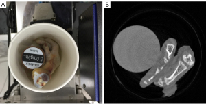
Figure 8 presents the reconstructed images and the corresponding gradient images of three representative energy bins (1st, 2nd and 4th). The results of SART are disturbed by noise, and image structures are destroyed. For the TV and TV+LR results (2nd and 3rd rows), the image noise is well suppressed by TV regularization. However, there are still blocky artifacts, and some details of the structures are lost. From the 4th and 5th rows, one can see the image quality of SSCMF and NLCTF methods are improved. Particularly, the NLCTF greatly preserves the image edges. Compared with the NLCTF, the reconstructed image quality of our IDEAS is further improved in image edge preservation and finer structures recovery.
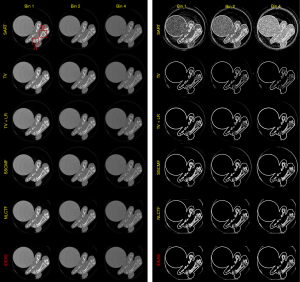
To further demonstrate the advantages of the proposed IDEAS method, Figure 9 displays magnified ROIs indicated by the red rectangle in Figure 8. From Figure 9, one can see that the SART, TV and TV+LR have a poor performance in all energy bins. The chicken foot contains complex structures that require advanced reconstruction algorithms to restore, the IDEAS may provide more accurate structural information than other competitors. The image structures indicated by the arrow “1” and “3” reconstructed by NLCTF are slightly lost, and these structures are over smoothed in the results of SSCMF, especially in high energy bins. However, in the IDEAS results, one can see more image structures are restored than the above two methods. Moreover, the image edges indicated by the arrow “2” of the SSCMF and NLCTF are blurred, and they are hardly observed in practice. On the contrary, the IDEAS can provide sharp image structure edges.
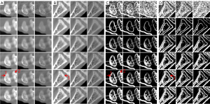
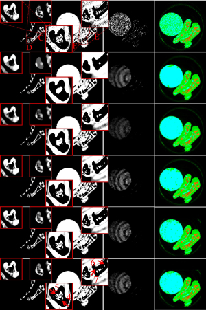
Figure 10 shows three basis material decomposition results from Figure 8. For the bone component in the 1st column of Figure 10, the developed IDEAS can produce much finer bone components information and obtain better edge structures than NLCTF, as indicated by the red ROIs “C” and “D”. For the soft-tissue component (2nd column), we can observe that some tiny soft tissue features indicated by the ROIs “E” and “F” are lost in the NLCTF, while the IDEAS result provides much more soft tissue structures. Regarding the iodine contrast component (3rd column), because the detector responses of this new PCD are not consistent, small ring artifact are still observable in the material images from all decomposition methods although the ring artifacts correction method has been used (49). From Figure 10, we can find that the comparison methods wrongly classify the pixels of bone component into iodine contrast, while NLCTF and IDEAS can provide more accurate iodine contrast images with less misclassification. In one word, all the material-specific images demonstrate that the IDEAS method can protect material edges and recovery finer structures very well compared with other methods.
Preclinical mouse study
To further demonstrate that IDEAS outperforms the competing methods, an anesthetized mouse is scanned by a state-of-the-art MARS multi-energy CT system (see Figure 11). The study was conducted in accordance with the laboratory animal guideline for ethical review of animal welfare and was approved by HKU Li Ka Shing Faculty of Medicine Ethics Committee for animal experiments. A flat-panel PCD is used. For the central slice, the PCD contains 600 detector elements and each of them covers a length of 0.11 mm. The emitting X-ray spectrum with 120 kVp is divided into five energy bins: [7.0, 32.0], [32.1, 43], [43.1, 54], [54.1, 70] and [70, 120]. The distances from the X-ray source to object and PCD are set as 15.6 and 25.6 cm, respectively. A total of 720 projections are uniformly collected in a full scan.
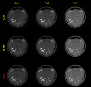
Figure 12 shows the reconstructed images of three representative energy bins (1st, 2nd and 5th). Since the NLCTF can obtain higher reconstructed accuracy than other competing methods, only the reconstructed results from SART, NLCTF and IDEAS methods are given in Figure 12 to save space. From Figure 12, one can see that the developed IDEAS technique has the best performance to recover fine structures and suppress noise-induced artifacts. The results of SART are disturbed by noise, and image structures are destroyed. Although the NLCTF can recover the structures, the reconstructed images contain noisy artifacts. Meanwhile, the results of NLCTF are tarnished by ring artifacts. The results of basis material decomposition are shown in Figure S1. The SART results have heavy noise and NLCTF results have severe image artifacts. The proposed IDEAS performs better than the competitors.
Discussion
The IDEAS involves non-local low-rank Tucker decomposition, multi-task TDL and weighted TV. All of those components make IDEAS different from the previously developed algorithms. Compared with NLCTF (25), IDEAS employs Tucker decomposition to replace KBR-based tensor decomposition, which is more flexible and computationally tractable. To encode nonlocal self-similarity characteristic, IDEAS employs the K-means++ clustering method to replace cube extraction and aggregation operation in NLCTF, which greatly reduces the computational complexity. Besides, IDEAS combines TDL and weighted TV while it inherits the non-local low-rank property of NLCTF. Compared with the TDL in our previous work (20), an effective multi-task TDL regularization with two different dictionaries is employed in a group of similar patches to further explore the sparsity, global correlation across the spectrum and nonlocal self-similarity characters. Specifically, two different dictionaries (spatial dictionary D1 and spectral dictionary D2) are used in the IDEAS. Different from other DL-based methods for multi-energy CT reconstruction (20,23), D1 and D2 are two small dictionaries that respectively control spatial and spectral properties. This can faithfully deliver the multi-factor affiliation underlying the multi-energy CT images. Besides, two different dictionaries in spatial and spectral dimensions are shared by all the tensor groups in the IDEAS. This means the features in space and spectrum can be learned from the whole image. Besides, the dictionaries are updated adaptively during an iterative reconstruction process, and they can reveal details which are invisible in the global DL reconstruction. Hence, it is necessary to use an adaptive dictionary when a global dictionary does not match a specific application closely (50). Compared with TV, IDEAS adopts weighted TV which can give different weighting parameters for channel-wise images.
While the IDEAS algorithm has superior performance for multi-energy CT reconstruction, there are still some open problems for practical applications. First, the proposed IDEAS algorithm contains several parameters that should be selected. The parameters are empirically selected based on quantitative index and visual evaluation. Note that, the parameters of all the competing methods had been carefully optimized based on the same strategies with IDEAS for a fair comparison. Even so, it still time-consuming to tune parameters, the strategy of parameters automatic optimization needs to be studied in the future. Second, the operations of clustering and tensor decomposition integrated in IDEAS are quite time-consuming. This can be accelerated by the graphics processing unit (GPU) techniques. Third, the proposed IDEAS assumes fan-beam CT geometry to demonstrate its merits in principle, and it can be directly generalized to a 4th-order tensor to deal with cone-beam CT or spiral CT for practical applications.
Acknowledgments
Funding: This work was supported in part by the National Natural Science Foundation of China (Nos. 62201616, 62101596, 62201628 and 61471070), and in part by the China Scholarship Council (No. 201906050067).
Footnote
Conflicts of Interest: All authors have completed the ICMJE uniform disclosure form (available at https://qims.amegroups.com/article/view/10.21037/qims-22-235/coif). The authors have no conflicts of interest to declare.
Ethical Statement: The authors are accountable for all aspects of the work in ensuring that questions related to the accuracy or integrity of any part of the work are appropriately investigated and resolved. The study was conducted in accordance with the laboratory animal guideline for ethical review of animal welfare and was approved by HKU Li Ka Shing Faculty of Medicine Ethics Committee for animal experiments.
Open Access Statement: This is an Open Access article distributed in accordance with the Creative Commons Attribution-NonCommercial-NoDerivs 4.0 International License (CC BY-NC-ND 4.0), which permits the non-commercial replication and distribution of the article with the strict proviso that no changes or edits are made and the original work is properly cited (including links to both the formal publication through the relevant DOI and the license). See: https://creativecommons.org/licenses/by-nc-nd/4.0/.
References
- So A, Nicolaou S. Spectral Computed Tomography: Fundamental Principles and Recent Developments. Korean J Radiol 2021;22:86-96. [Crossref] [PubMed]
- Wang Y, Cai A, Liang N, Yu X, Zhong X, Li L, Yan B. One half-scan dual-energy CT imaging using the Dual-domain Dual-way Estimated Network (DoDa-Net) model. Quant Imaging Med Surg 2022;12:653-74. [Crossref] [PubMed]
- Wen Q, Yue Y, Shang J, Lu X, Gao L, Hou Y. The application of dual-layer spectral detector computed tomography in solitary pulmonary nodule identification. Quant Imaging Med Surg 2021;11:521-32. [Crossref] [PubMed]
- Kim K, Ye JC, Worstell W, Ouyang J, Rakvongthai Y, El Fakhri G, Li Q. Sparse-view spectral CT reconstruction using spectral patch-based low-rank penalty. IEEE Trans Med Imaging 2015;34:748-60. [Crossref] [PubMed]
- Alvarez RE, Seibert JA, Thompson SK. Comparison of dual energy detector system performance. Med Phys 2004;31:556-65. [Crossref] [PubMed]
- Wu W, Hu D, An K, Wang S, Luo F. A high-quality photon-counting CT technique based on weight adaptive total-variation and image-spectral tensor factorization for small animals imaging. IEEE Trans Instrum Meas 2020;70:1-14.
- He P, Wei B. Med Phys 2012;39:6572-9. [Crossref] [PubMed]
- Wang S, Wu W, Feng J, Liu F, Yu H. Low-dose spectral CT reconstruction based on image-gradient L0-norm and adaptive spectral PICCS. Phys Med Biol 2020;65:245005. [Crossref] [PubMed]
- Feng J, Yu H, Wang S, Liu F. Image-domain based material decomposition by multi-constraint optimization for spectral CT. IEEE Access 2020;8:155450-8.
- Walsh MF, Opie AMT, Ronaldson JP, Doesburg RMN, Nik SJ, Mohr JL, Ballabriga R, Butler APH, Butler PH. First CT using Medipix3 and the MARS-CT-3 spectral scanner. Journal of Instrumentation 2011;6:C01095. [Crossref]
- Xu Q, Yu H, Bennett J, He P, Zainon R, Doesburg R, Opie A, Walsh M, Shen H, Butler A, Butler P, Mou X, Wang G. Image reconstruction for hybrid true-color micro-CT. IEEE Trans Biomed Eng 2012;59:1711-9. [Crossref] [PubMed]
- Zhao B, Ding H, Lu Y, Wang G, Zhao J, Molloi S. Dual-dictionary learning-based iterative image reconstruction for spectral computed tomography application. Phys Med Biol 2012;57:8217-29. [Crossref] [PubMed]
- Zhang Y, Xi Y, Yang Q. IEEE Trans Comput Imaging 2016;2:510-23. [Crossref] [PubMed]
- Wang M, Zhang Y, Liu R, Guo S, Yu H. An adaptive reconstruction algorithm for spectral CT regularized by a reference image. Phys Med Biol 2016;61:8699-719. [Crossref] [PubMed]
- Yu Z, Leng S, Li Z, McCollough CH. Spectral prior image constrained compressed sensing (spectral PICCS) for photon-counting computed tomography. Phys Med Biol 2016;61:6707-32. [Crossref] [PubMed]
- Yu H, Wu W, Chen P, Gong C, Jiang J, Wang S, Liu F, Yu H. Image gradient L0-norm based PICCS for swinging multi-source CT reconstruction. Opt Express 2019;27:5264-79. [Crossref] [PubMed]
- Chu J. Phys Med Biol 2013;58:7009-24. [Crossref] [PubMed]
- Gao H, Yu H, Osher S, Wang G. Multi-energy CT based on a prior rank, intensity and sparsity model (PRISM). Inverse Probl 2011; [Crossref] [PubMed]
- Semerci O, Hao Ning, Kilmer ME, Miller EL. Tensor-based formulation and nuclear norm regularization for multienergy computed tomography. IEEE Trans Image Process 2014;23:1678-93. [Crossref] [PubMed]
- Zhang Y, Mou X, Wang G, Yu H. Tensor-Based Dictionary Learning for Spectral CT Reconstruction. IEEE Trans Med Imaging 2017;36:142-54. [Crossref] [PubMed]
- Wu W, Zhang Y, Wang Q, Liu F, Chen P, Yu H. Low-dose spectral CT reconstruction using image gradient ℓ 0-norm and tensor dictionary. Appl Math Model 2018;63:538-57. [Crossref] [PubMed]
- Xu M, Hu D, Luo F, Liu F, Wang S, Wu W. Limited-angle X-ray CT reconstruction using image gradient ℓ0-norm with dictionary learning. IEEE Trans Radiat Plasma Med Sci 2020;5:78-87. [Crossref]
- Hu D, Wu W, Xu M, Zhang Y, Liu J, Ge R, Chen Y, Luo L, Coatrieux G. SISTER: Spectral-Image Similarity-Based Tensor With Enhanced-Sparsity Reconstruction for Sparse-View Multi-Energy CT. IEEE Trans Comput Imaging 2019;6:477-90. [Crossref]
- Wu W, Zhang Y, Wang Q, Liu F, Luo F, Yu H. Spatial-Spectral Cube Matching Frame for Spectral CT Reconstruction. Inverse Probl 2018;34:104003. [Crossref] [PubMed]
- Wu W, Liu F, Zhang Y, Wang Q, Yu H. Non-Local Low-Rank Cube-Based Tensor Factorization for Spectral CT Reconstruction. IEEE Trans Med Imaging 2019;38:1079-93. [Crossref] [PubMed]
- Wu W, Guo X, Chen Y, Wang S, Chen J. Deep Embedding-Attention-Refinement for Sparse-view CT Reconstruction. IEEE Trans Instrum Meas 2022; [Crossref]
- Wang S, Yu H, Xi Y, Gong C, Wu W, Liu F. Spectral-image decomposition with energy-fusion sensing for spectral CT reconstruction. IEEE Trans Instrum Meas 2021;70:1-11. [Crossref]
- Zimichev EA, Kazanskii NL, Serafimovich PG. Spectral-spatial classification with k-means++ particional clustering. Computer Optics 2014;38:281-6. [Crossref]
- Liu Y, Long Z, Huang H, Zhu C. Low CP rank and Tucker rank tensor completion for estimating missing components in image data. IEEE Trans Circuits Syst Video Technol 2019;30:944-54. [Crossref]
- Tan S, Zhang Y, Wang G, Mou X, Cao G, Wu Z, Yu H. Tensor-based dictionary learning for dynamic tomographic reconstruction. Phys Med Biol 2015;60:2803-18. [Crossref] [PubMed]
- Liu Y, Chen L, Zhu C. Improved robust tensor principal component analysis via low-rank core matrix. IEEE J Sel Top Signal Process 2018;12:1378-89. [Crossref]
- Zeng D, Xie Q, Cao W, Lin J, Zhang H, Zhang S, Huang J, Bian Z, Meng D, Xu Z, Liang Z, Chen W, Ma J. Low-Dose Dynamic Cerebral Perfusion Computed Tomography Reconstruction via Kronecker-Basis-Representation Tensor Sparsity Regularization. IEEE Trans Med Imaging 2017;36:2546-56. [Crossref] [PubMed]
- Long Z, Liu Y, Chen L, Zhu C. Low rank tensor completion for multiway visual data. Signal Processing 2019;155:301-16. [Crossref]
- De Lathauwer L, De Moor B, Vandewalle J. A multilinear singular value decomposition. SIAM journal on Matrix Analysis Applications 2000;21:1253-78. [Crossref]
- De Lathauwer L, De Moor B, Vandewalle J. On the best rank-1 and rank-(r 1, r 2, rn) approximation of higher-order tensors. SIAM Journal on Matrix Analysis Applications 2000;21:1324-42. [Crossref]
- Wu W, Hu D, Cong W, Shan H, Wang S, Niu C, Yan P, Yu H, Vardhanabhuti V, Wang G. Stabilizing deep tomographic reconstruction: Part A. Hybrid framework and experimental results. Patterns (N Y) 2022;3:100474.
- Wu W, Hu D, Cong W, Shan H, Wang S, Niu C, Yan P, Yu H, Vardhanabhuti V, Wang G. Stabilizing deep tomographic reconstruction: Part B. Convergence analysis and adversarial attacks. Patterns (N Y) 2022;3:100475.
- Goldstein T, Osher S. The split Bregman method for L1-regularized problems. SIAM Journal on Imaging Sciences 2009;2:323-43. [Crossref]
- Lee H, Battle A, Raina R, Ng A. Efficient sparse coding algorithms. In: Schölkopf B, Platt J, Hofmann T. editors. Advances in Neural Information Processing Systems 19: Proceedings of the 2006 Conference. MIT Press, 2016.
- Peng Y, Meng D, Xu Z, Gao C, Yang Y, Zhang B. Decomposable nonlocal tensor dictionary learning for multispectral image denoising. 2014 IEEE Conference on Computer Vision and Pattern Recognition; 23-28 June 2014; Columbus, OH, USA. IEEE, 2014.
- Segars WP, Tsui BM, Frey EC, Johnson GA, Berr SS. Development of a 4-D digital mouse phantom for molecular imaging research. Mol Imaging Biol 2004;6:149-59. [Crossref] [PubMed]
- Ronaldson J, Walsh M, Nik S, Donaldson J, Doesburg R, van Leeuwen D, Ballabriga R, Clyne M, Butler A, Butler P. Characterization of Medipix3 with the MARS readout and software. Journal of Instrumentation 2011;6:C01056. [Crossref]
- Wang Z, Bovik AC, Sheikh HR, Simoncelli EP. Image quality assessment: from error visibility to structural similarity. IEEE Trans Image Process 2004;13:600-12. [Crossref] [PubMed]
- Wu W, Chen P, Wang S, Vardhanabhuti V, Liu F, Yu H. Image-domain Material Decomposition for Spectral CT using a Generalized Dictionary Learning. IEEE Trans Radiat Plasma Med Sci 2021;5:537-47. [Crossref] [PubMed]
- Zhang T, Yu H, Xi Y, Wang S, Liu F, Spectral CT. Image-domain Material Decomposition via Sparsity Residual Prior and Dictionary Learning. IEEE Trans Instrum Meas 2022; [Crossref]
- Badea CT, Johnston SM, Qi Y, Ghaghada K, Johnson GA. Dual-energy micro-CT imaging for differentiation of iodine- and gold-based nanoparticles. Proceedings of SPIE the International Society for Optical Engineering 2011;7961.
- Liu X, Yu L, Primak AN, McCollough CH. Quantitative imaging of element composition and mass fraction using dual-energy CT: three-material decomposition. Med Phys 2009;36:1602-9. [Crossref] [PubMed]
- Fredette NR, Kavuri A, Das M. Multi-step material decomposition for spectral computed tomography. Phys Med Biol 2019;64:145001. [Crossref] [PubMed]
- Chang S, Chen X, Duan J, Mou X. A CNN-Based Hybrid Ring Artifact Reduction Algorithm for CT Images. IEEE Trans Radiat Plasma Med Sci 2020;5:253-60. [Crossref]
- Yu H, Wang S, Wu W, Gong C, Wang L, Pi Z, Liu F. Weighted adaptive non-local dictionary for low-dose CT reconstruction. Signal Processing 2021;180:107871. [Crossref]


